Full-Field Inference: Implicit vs Explicit approaches
Cosmology in the Adriatic -- From PT to AI, July 2024
François Lanusse

slides at eiffl.github.io/talks/Split2024
Full-Field Simulation-Based Inference
- Instead of trying to analytically evaluate the likelihood of
sub-optimal summary statistics, let us build a forward model of the full observables.
$\Longrightarrow$ The simulator becomes the physical model. - Each component of the model is now tractable, but at the cost of a large number of latent variables.
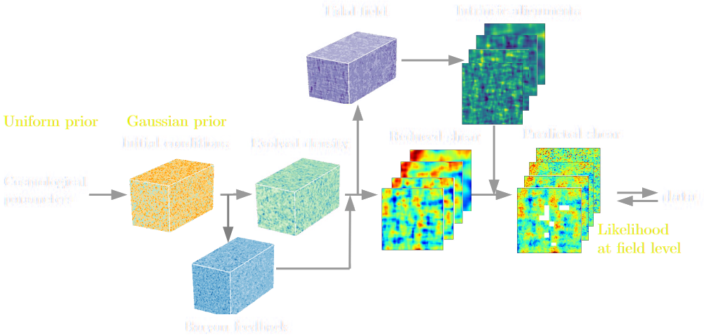
Benefits of a forward modeling approach
- Fully exploits the information content of the data (aka "full field inference").
- Easy to incorporate systematic effects.
- Easy to combine multiple cosmological probes by joint simulations.
(Porqueres et al. 2021)
For this talk, let's ignore the elephant in the room:
Do we have reliable enough models for the full complexity of the data?
Do we have reliable enough models for the full complexity of the data?
...so why is this not completely mainstream?
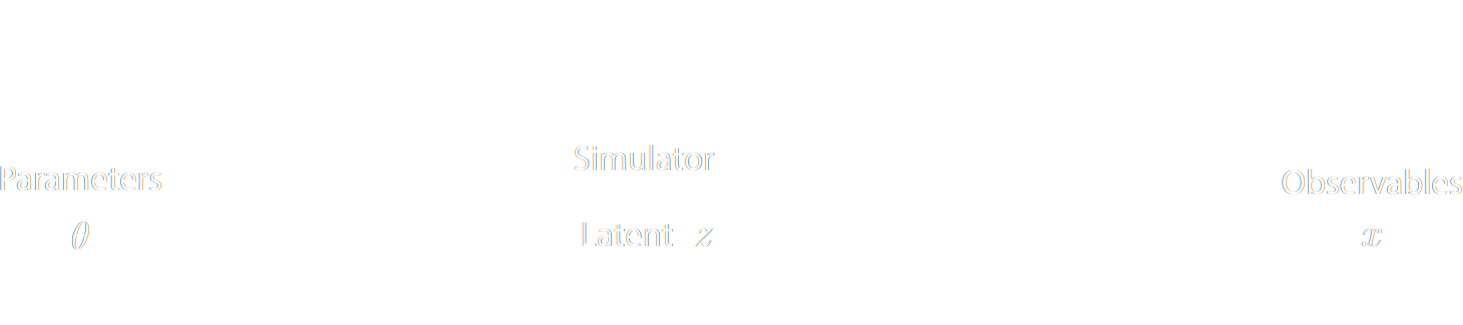
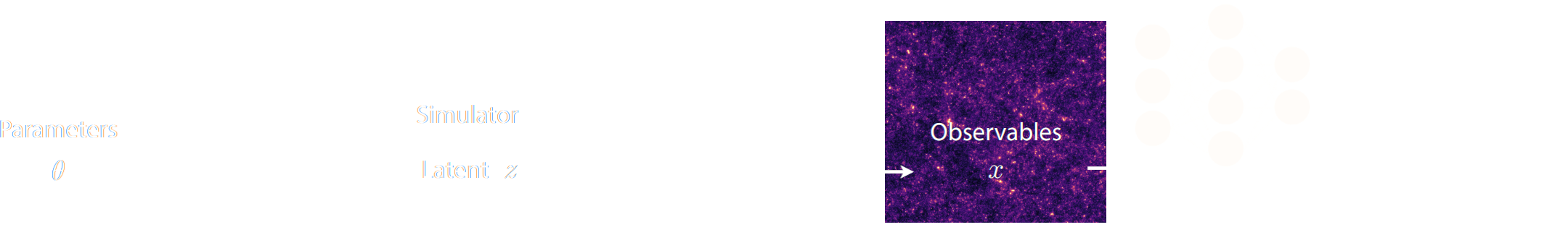
The Challenge of Simulation-Based Inference
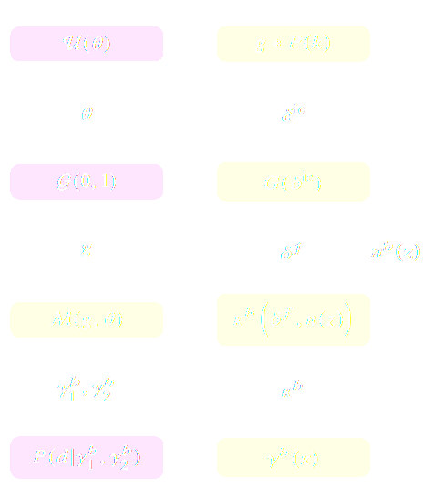
$$ p(x|\theta) = \int p(x, z | \theta) dz = \int p(x | z, \theta) p(z | \theta) dz $$
Where $z$ are stochastic latent variables of the simulator.
$\Longrightarrow$ This marginal likelihood is intractable!
$\Longrightarrow$ This marginal likelihood is intractable!
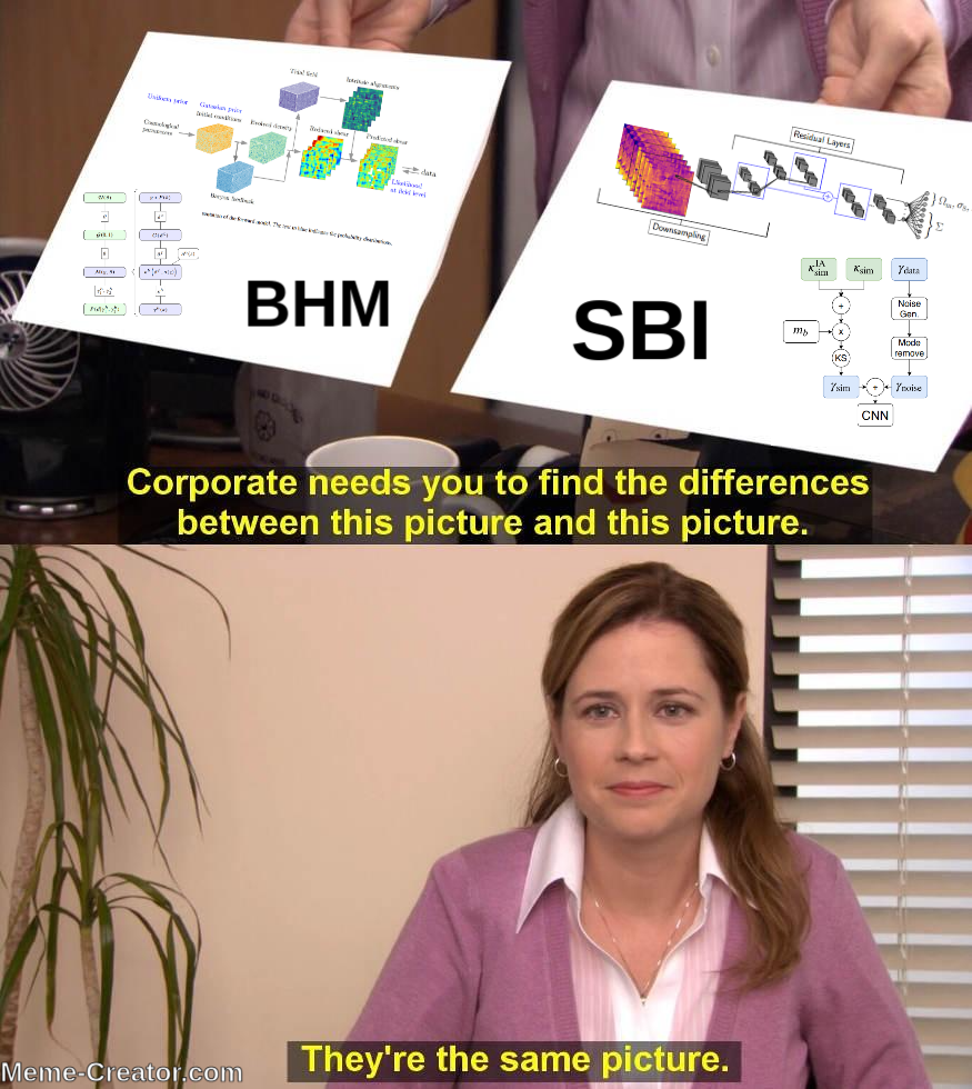
How to perform inference over forward simulation models?
- Implicit Inference: Treat the simulator as a black-box with only the ability to sample from the joint distribution
$$(x, \theta) \sim p(x, \theta)$$
a.k.a.
- Simulation-Based Inference (SBI)
- Likelihood-free inference (LFI)
- Approximate Bayesian Computation (ABC)
- Explicit Inference: Treat the simulator as a probabilistic model and perform inference over the joint posterior
$$p(\theta, z | x) \propto p(x | z, \theta) p(z, \theta) p(\theta) $$
a.k.a.
- Bayesian Hierarchical Modeling (BHM)
$\Longrightarrow$ For a given simulation model, both methods should converge to the same posterior!
Main Questions for This Talk
- Do we have the practical methodologies for both form of inference
that converge to the same solution?
- What is the tradeoff in computational cost between the two approaches?
Optimal Neural Summarisation for Full-Field Weak Lensing Cosmological Implicit Inference
Work led by:
Denise Lanzieri (now at Sony Computer Science Laboratory)
Justine Zeghal (moving to University of Montreal in the fall)


$\Longrightarrow$ Compare strategies for neural compression in setting where explicit posterior is available.
Conventional Recipe for Full-Field Implicit Inference...
A two-steps approach to Implicit Inference
- Automatically learn an optimal low-dimensional summary statistic $$y = f_\varphi(x) $$
- Use Neural Density Estimation to either:
- build an estimate $p_\phi$ of the likelihood function $p(y \ | \ \theta)$ (Neural Likelihood Estimation)
- build an estimate $p_\phi$ of the posterior distribution $p(\theta \ | \ y)$ (Neural Posterior Estimation)
But a lot of variants!
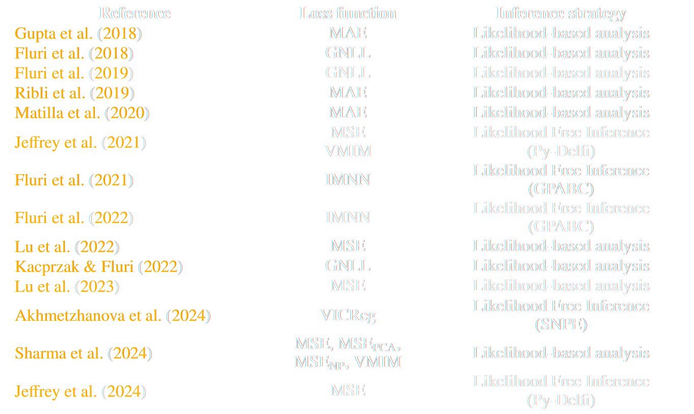
* grey rows are papers analyzing survey data
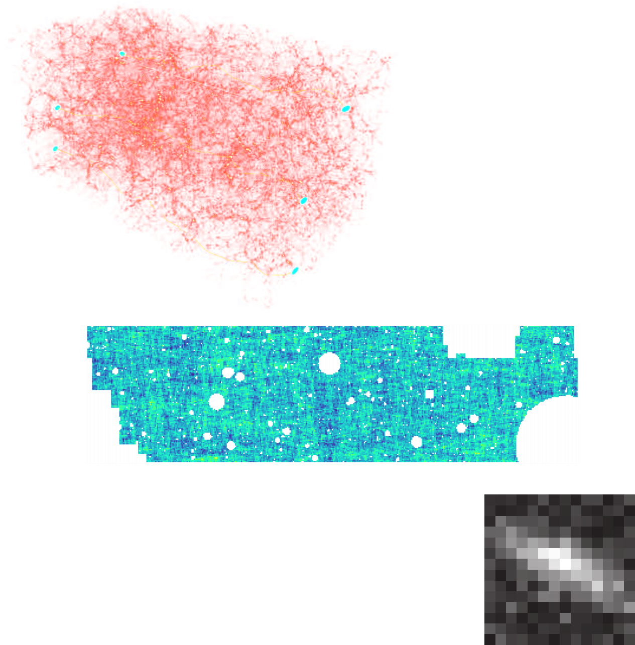
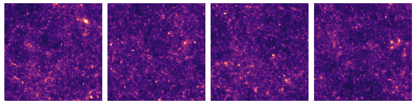
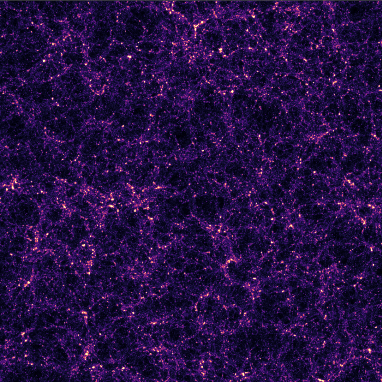
An easy-to-use experimentation testbed: log-normal lensing simulations

DifferentiableUniverseInitiative/sbi_lens
JAX-based log-normal lensing simulation package
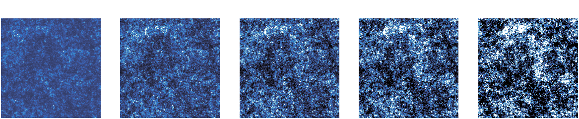
- 10x10 deg$^2$ maps at LSST Y10 quality, conditioning the log-normal shift parameter on $(\Omega_m, \sigma_8, w_0)$
- Provides explicit posterior by Hamiltonian-Monte Carlo (NUTS) sampling in reasonable time
- Can be used to sample a practically infinite number of maps for implicit inference
Information Point of View on Neural Summarisation
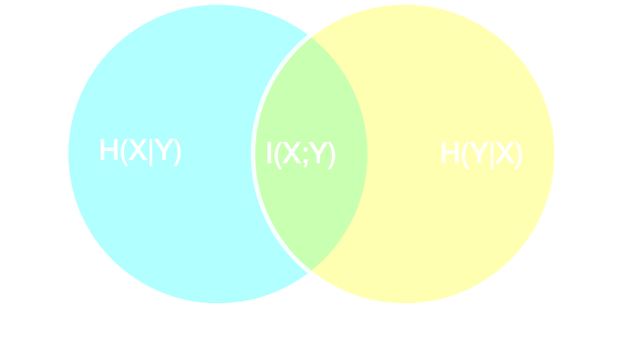
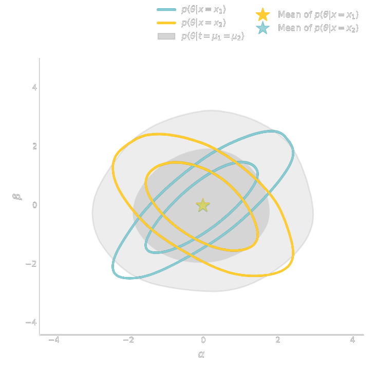
Learning Sufficient Statistics
- Summary statistics $y$ is sufficient for $\theta$ if $$ I(Y; \Theta) = I(X; \Theta) \Leftrightarrow p(\theta | x ) = p(\theta | y) $$
- Variational Mutual Information Maximization
$$ \mathcal{L} \ = \ \mathbb{E}_{x, \theta} [ \log q_\phi(\theta | y=f_\varphi(x)) ] \leq I(Y; \Theta) $$
(Barber & Agakov variational lower bound)
Jeffrey, Alsing, Lanusse (2021)

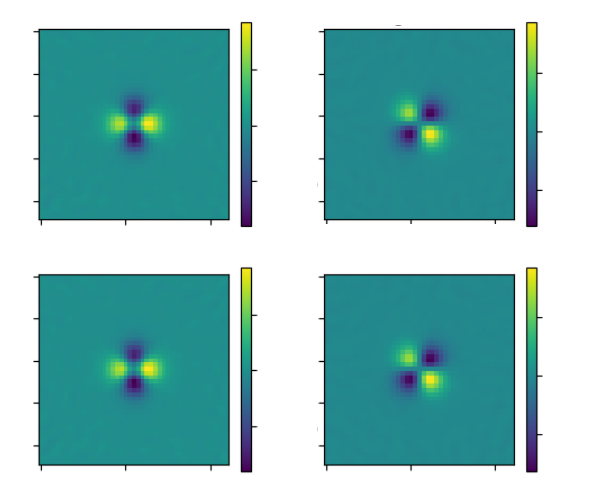
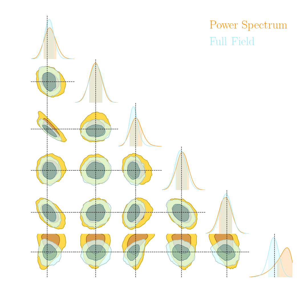
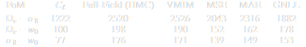
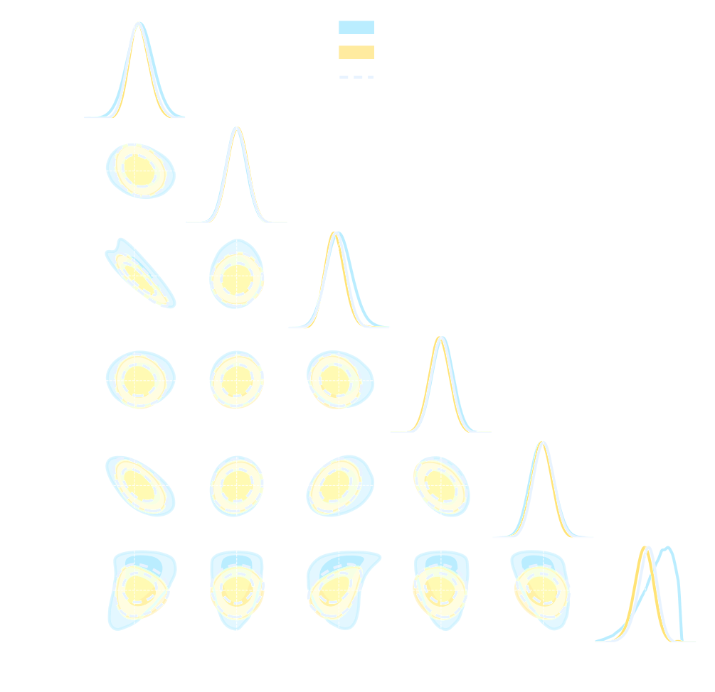
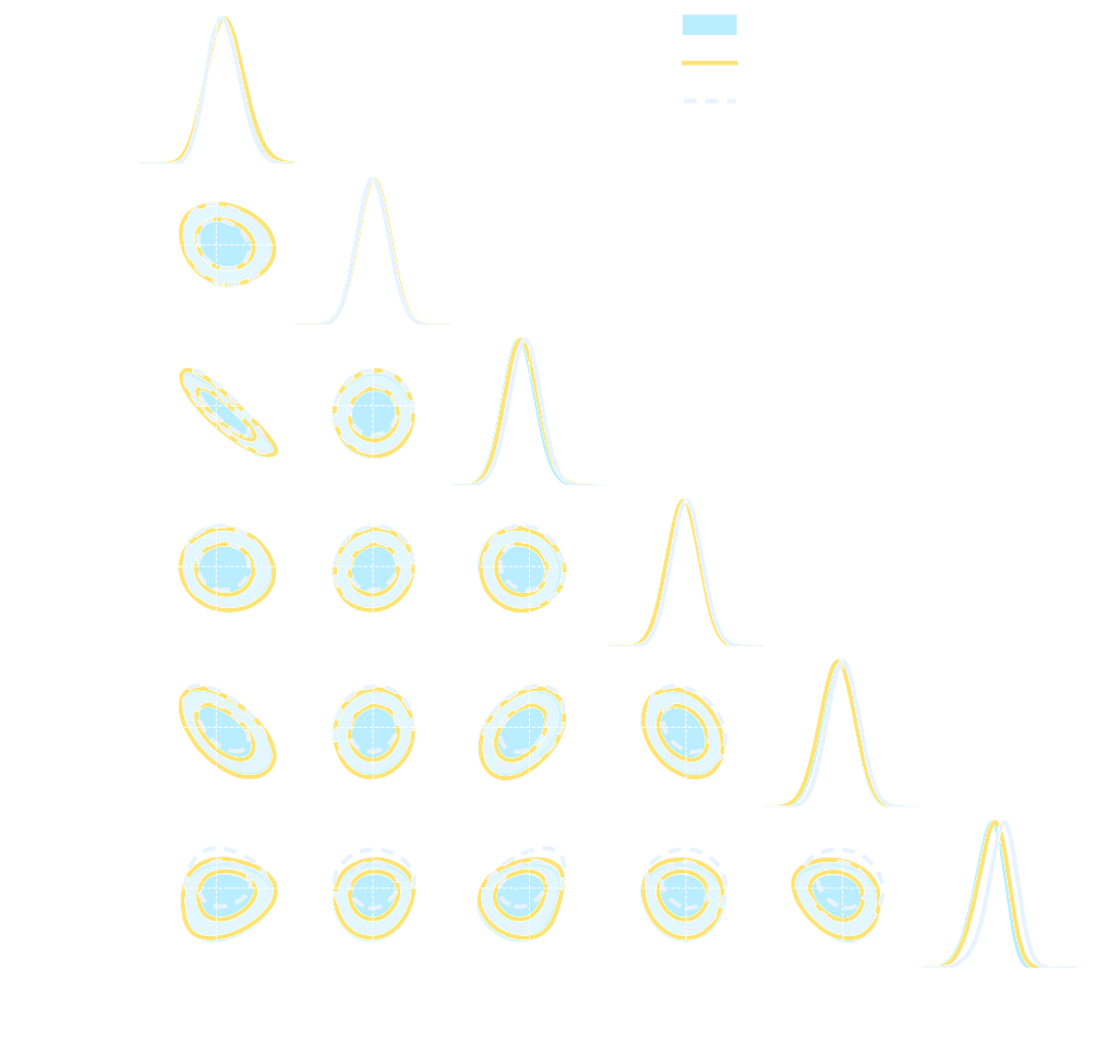
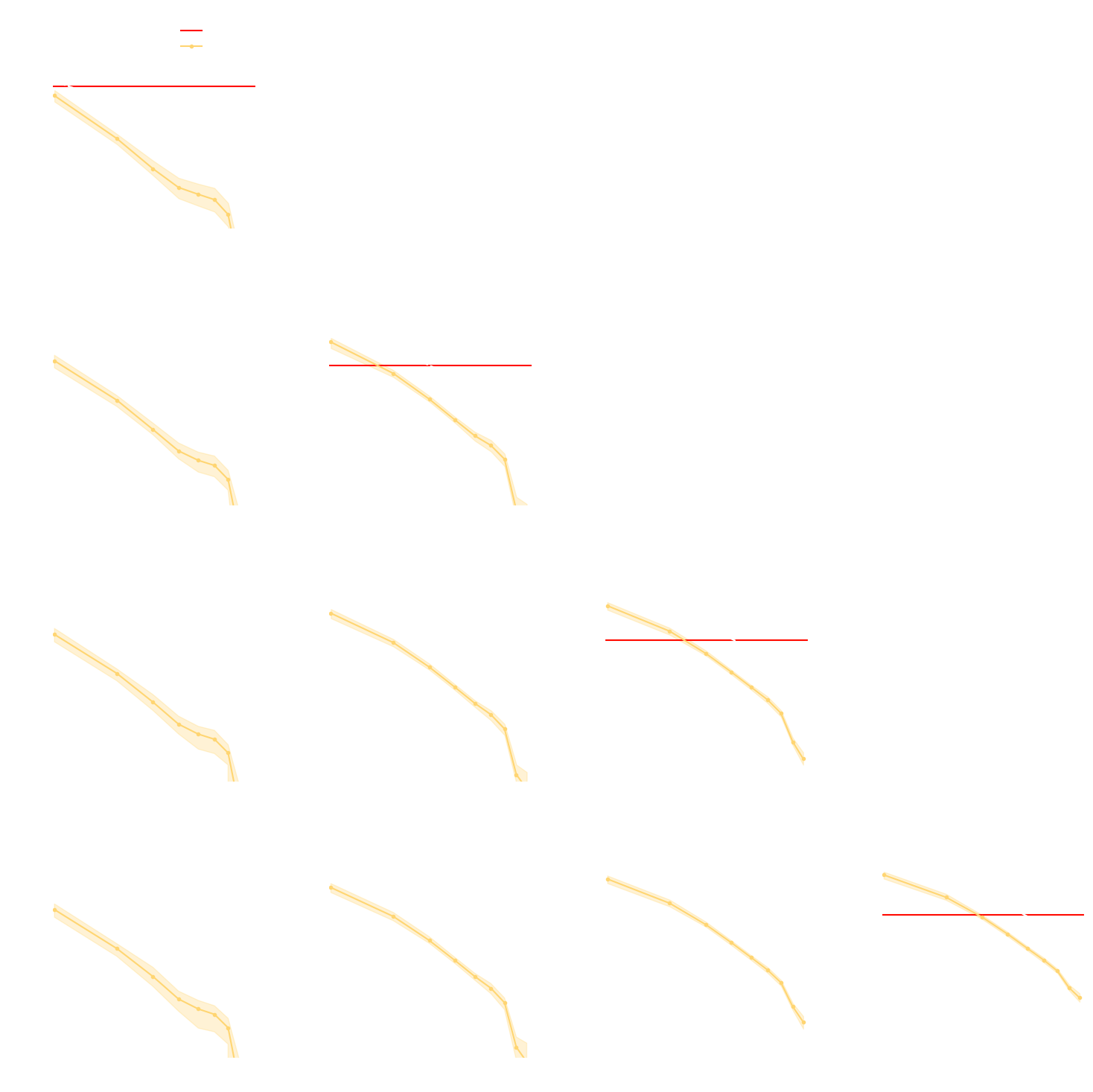
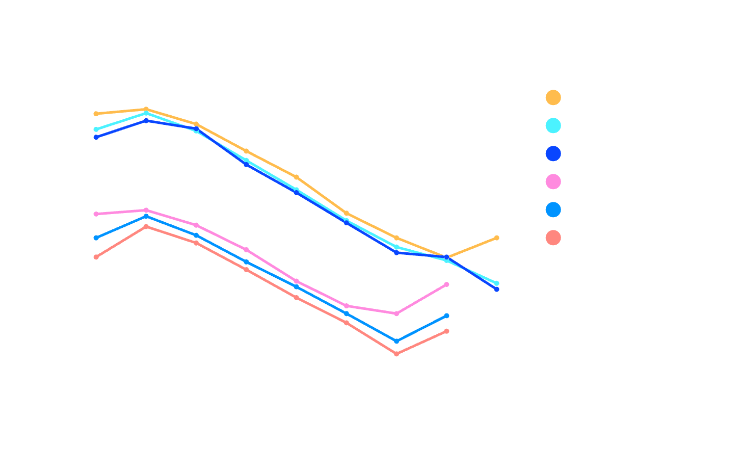
Main takeaways
- Asymptotically VMIM yields a sufficient statistics
- No reason not to use it in practice, it works well, and is asymptotically optimal
- Mean Squared Error (MSE) DOES NOT yield a sufficient statistics even asymptotically
- Same for Mean Absolute Error (MAE) and weighted versions of MSE
![]()
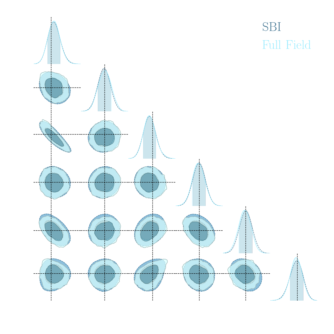
- Spoiler: in upcoming LSST DESC paper (Zeghal et al., in prep.) we report that in this setting:
- Explicit inference converges in $O(10^6)$ model evaluations.
- Implicit Inference converges in $O(10^3)$ model evaluations at fixed summary statistics.
credit: Justine Zeghal
Implicit Inference is easier, cheaper, and yields the same results as Explicit Inference...
But Explicit Inference is cooler, so can we do it anyway?
Credit: Yuuki Omori, Chihway Chang, Justine Zeghal, EiffL
https://github.com/EiffL/LPTLensingComparison
More seriously, Explicit Inference has some advantages:
- More introspectable results to identify systematics
- Allows for fitting parametric corrections/nuisances from data
- Provides validation of statistical inference with a different method
Automatically Differentiable High Performance Computing
Work led by:
Wassim Kabalan (PhD Student at IN2P3/APC)

$\Longrightarrow$ Build near compute-optimal distributed simulators in JAX on GPU-based supercomputers
State of the art of differentiable lensing model (Porqueres et al. 2023)
 Settings:
 - 1LPT lightcone
- (1 x 1 x 4.5) $h^{-1}$Gpc
- 64 x 64 x 128 voxels
- 16 x 16 degrees lensing field
- ~2 hours to sample with NUTS on one A100
(our implementation)
Comparison to linear lensing power spectra
$\Longrightarrow$ We need to go bigger!
Mesh FlowPM: Distributed and Automatically Differentiable simulations
Modi, Lanusse, Seljak (2020)

- We developed a Mesh TensorFlow implementation that can scale on GPU clusters.
- Based on low-level NVIDIA NCCL collectives, accessed through Horovod.
- For a $2048^3$ simulation:
- Distributed on 256 NVIDIA V100 GPUs on the Jean Zay supercomputer
- Runtime: ~3 mins
- This is great... but Mesh TensorFlow is now abandonned.
Towards a new generation of JAX-based distributed tools
- JAX v0.4.1 (Dec. 2022) has made a strong push for bringing automated parallelization and support multi-host GPU clusters!
- Scientific HPC still most likely requires dedicated high-performance ops
- jaxDecomp: Domain Decomposition and Parallel FFTs
![]()
- JAX bindings to the high-performance cuDecomp (Romero et al. 2022) adaptive domain decomposition library.
- Provides parallel FFTs and halo-exchange operations.
- Supports variety of backends: CUDA-aware MPI, NVIDIA NCCL, NVIDIA NVSHMEM.
Defining Custom Distributed Ops in JAX
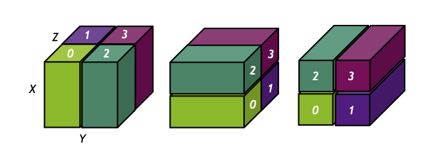
	from jax.experimental import mesh_utils
	from jax.sharding import PositionalSharding

	# Create a Sharding object to distribute a value across devices:
	sharding = PositionalSharding(mesh_utils.create_device_mesh((8,)))

	# Create an array of random values:
	x = jax.random.normal(jax.random.PRNGKey(0), (8192, 8192))
	# and use jax.device_put to distribute it across devices:
	y = jax.device_put(x, sharding.reshape(4, 2))
	jax.debug.visualize_array_sharding(y)

	---

	┌──────────┬──────────┐
	│  TPU 0   │  TPU 1   │
	├──────────┼──────────┤
	│  TPU 2   │  TPU 3   │
	├──────────┼──────────┤
	│  TPU 6   │  TPU 7   │
	├──────────┼──────────┤
	│  TPU 4   │  TPU 5   │
	└──────────┴──────────┘
	from jaxlib.hlo_helpers import custom_call

	def _rms_norm_fwd_cuda_lowering(ctx, x, weight, eps):
		[...]
		opaque = gpu_ops.create_rms_norm_descriptor([...])

		out = custom_call(
			b"rms_forward_affine_mixed_dtype",
			result_types=[
				ir.RankedTensorType.get(x_shape, w_type.element_type),
				ir.RankedTensorType.get((n1,), iv_element_type),
			],
			operands=[x, weight],
			backend_config=opaque,
			operand_layouts=default_layouts(x_shape, w_shape),
			result_layouts=default_layouts(x_shape, (n1,)),
		).results
		return out

	_rms_norm_fwd_p = core.Primitive("rms_norm_fwd")
	mlir.register_lowering(
		_rms_norm_fwd_p,
		_rms_norm_fwd_cuda_lowering,
		platform="gpu",
	)
						def partition(mesh, arg_shapes, result_shape):
							result_shardings = jax.tree.map(lambda x: x.sharding, result_shape)
							arg_shardings = jax.tree.map(lambda x: x.sharding, arg_shapes)
							return mesh, fft, \
								supported_sharding(arg_shardings[0], arg_shapes[0]), \
								(supported_sharding(arg_shardings[0], arg_shapes[0]),)

						def infer_sharding_from_operands(mesh, arg_shapes, result_shape):
							arg_shardings = jax.tree.map(lambda x: x.sharding, arg_shapes)
							return supported_sharding(arg_shardings[0], arg_shapes[0])

						@custom_partitioning
						def my_fft(x):
							return fft(x)

						my_fft.def_partition(
							infer_sharding_from_operands=infer_sharding_from_operands,
							partition=partition)
JAX cuDecomp interface led by Wassim Kabalan (IN2P3/APC)
- JAX>=v0.4.1 defines sharded tensors and a "computation follows data" philosophy.
- jaxlib provides a helper to define custom CUDA lowering
- Recent API allows us to define custom partitioning schemes compatible with a primitive
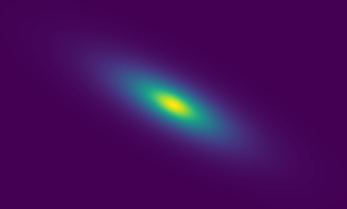
Building PM components from these distributed operations
Kabalan, Lanusse, Boucaud (in prep.)
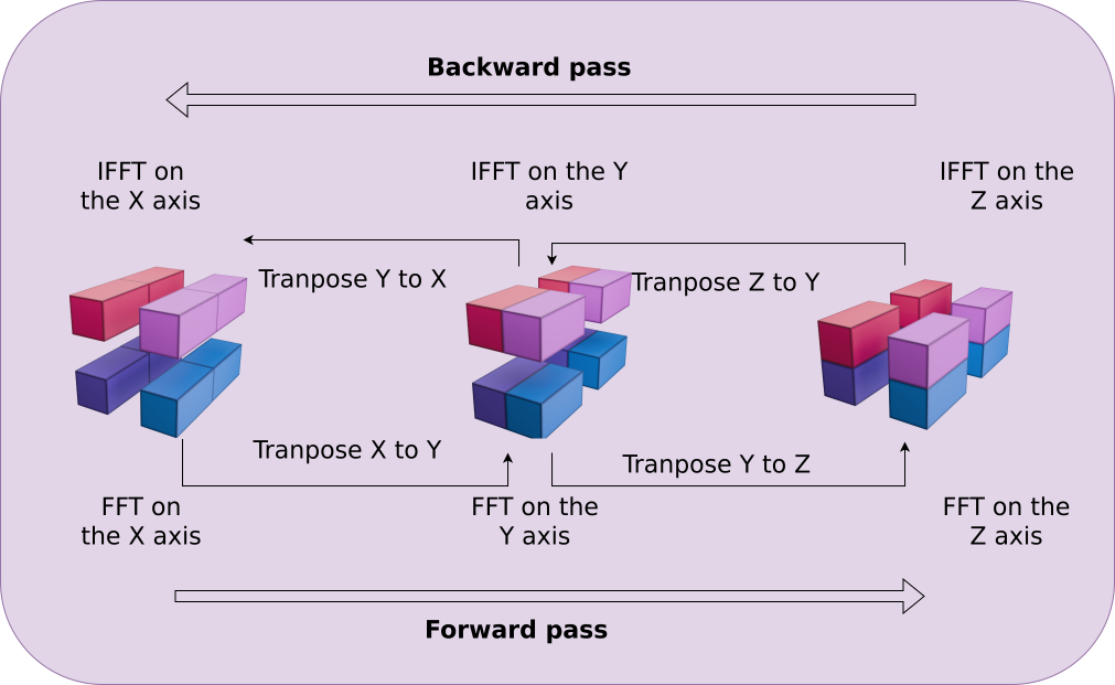
Distributed 3D FFT for force computation
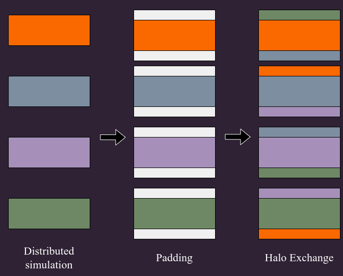
Halo Exchange for CiC painting and reading
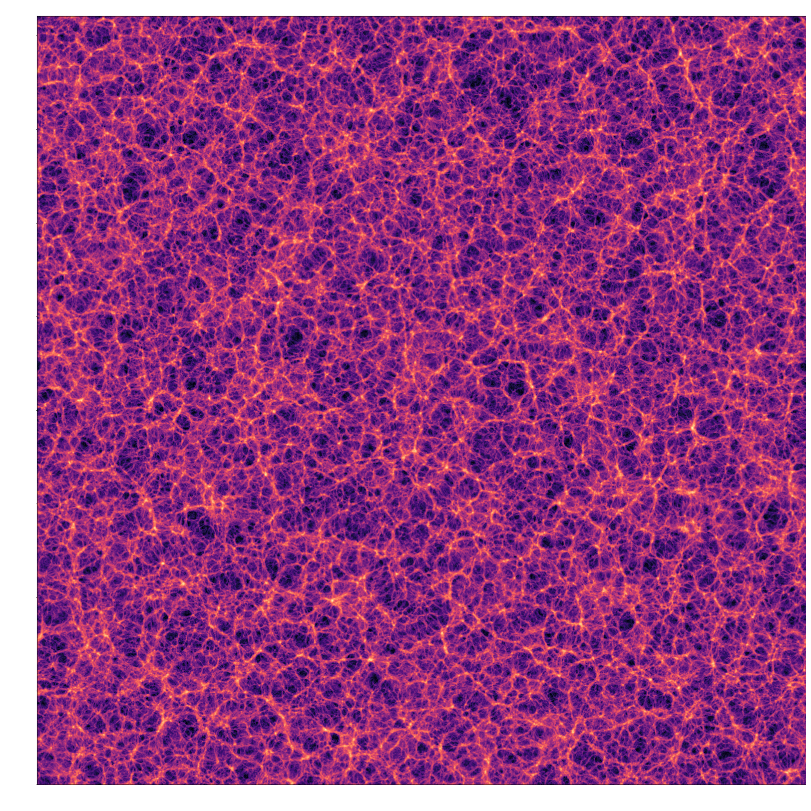
$2048^3$ LPT field, 1.02s on 32 H100 GPUs
Performance Benchmark
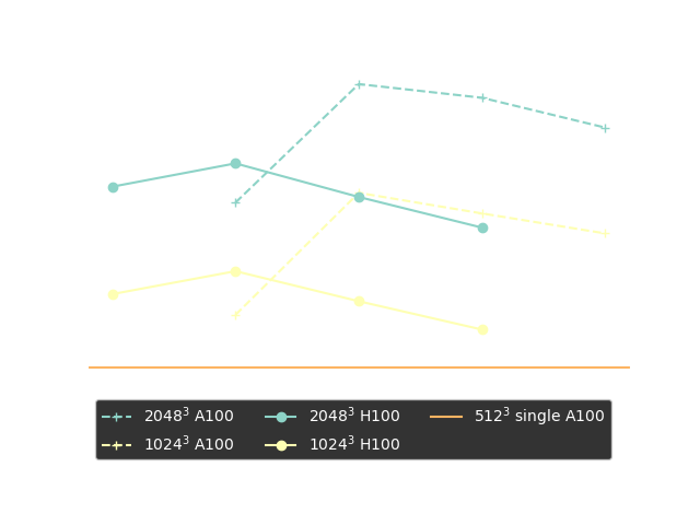
Strong scaling plots of 3D FFT
Official performance benchmark from NVIDIA with cuFFTMp
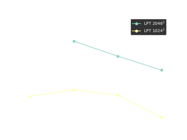
Timing of 1LPT computation
On the topic of JAX codes...
Jax-GalSim: it's GalSim, but Differentiable and GPU-accelerated!
						import jax_galsim as galsim

						psf_beta = 5       #
						psf_re = 1.0       # arcsec
						pixel_scale = 0.2  # arcsec / pixel
						sky_level = 2.5e3  # counts / arcsec^2

						# Define the galaxy profile.
						gal = galsim.Exponential(flux=1, scale_radius=2).shear(g1=.3, g2=.4)
						gal = gal.shear(g1=0.01, g2=0.05)

						# Define the PSF profile.
						psf = galsim.Gaussian(flux=1., half_light_radius=psf_re)

						# Final profile is the convolution of these.
						final = galsim.Convolve([gal, psf])

						# Draw the image with a particular pixel scale.
						image = final.drawImage(scale=pixel_scale)
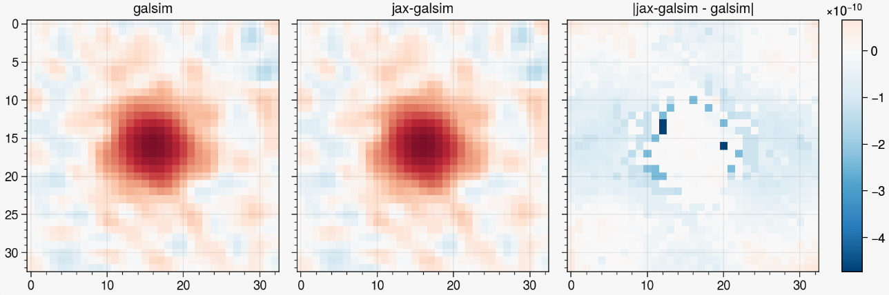
metacalibration residuals, credit: Matt Becker
Guiding principles:
- Strictly follows the GalSim API.
- Validated against GalSim up to numerical accuracy: inherits from GalSim's test suite
- Implementations should be easy to read and understand.
Example use-case: Metacalibration in 3 lines of code!
						@jax.jacfwd
						def autometacal(shear, image, psf, rec_psf):
							# Step 1: Deconvolve the image
							deconvolved = jax_galsim.Convolve([image,
																		jax_galsim.Deconvolve(psf)])
							# Step 2: Apply shear
							sheared = deconvolved.shear(g1=shear[0], g2=shear[1])
							# Step 3: Reconvolve by slightly dilated PSF
							reconvolve = jax_galsim.Convolve([sheared, rec_psf])
							return reconvolve.drawImage(scale=scale, method='no_pixel').array