Deep Learning for Observational Cosmology
N3AS Summer School, Santa Cruz, July 2023
François Lanusse


slides at eiffl.github.io/talks/SantaCruz2023
a new era of wide-field galaxy surveys


One of the core probes: gravitational lensing
Galaxy shapes as estimators for gravitational shear
$$ e = \gamma + e_i \qquad \mbox{ with } \qquad e_i \sim \mathcal{N}(0, I)$$
- We are trying the measure the ellipticity $e$ of galaxies as an estimator for the gravitational shear $\gamma$
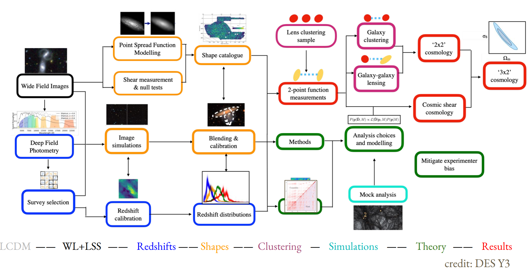
Illustration on the Dark Energy Survey (DES) Y3
Jeffrey, et al. (2021)
The DES Y3 pipeline
the Rubin Observatory Legacy Survey of Space and Time
- 1000 images each night, 15 TB/night for 10 years
- 18,000 square degrees, observed once every few days
- Tens of billions of objects, each one observed $\sim1000$ times
Previous generation survey: SDSS
Image credit: Peter Melchior
Current generation survey: DES
Image credit: Peter Melchior
LSST precursor survey: HSC
Image credit: Peter Melchior
The challenges of modern surveys
$\Longrightarrow$ Modern surveys will provide large volumes of high quality data
A Blessing
- Unprecedented statistical power
- Great potential for new discoveries
A Curse
- Existing methods are reaching their limits at every step of the science analysis
- Control of systematics is paramount
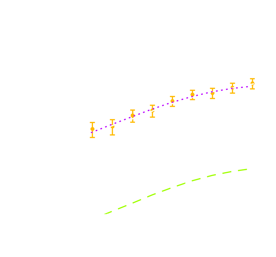
LSST forecast on dark energy parameters
![]()
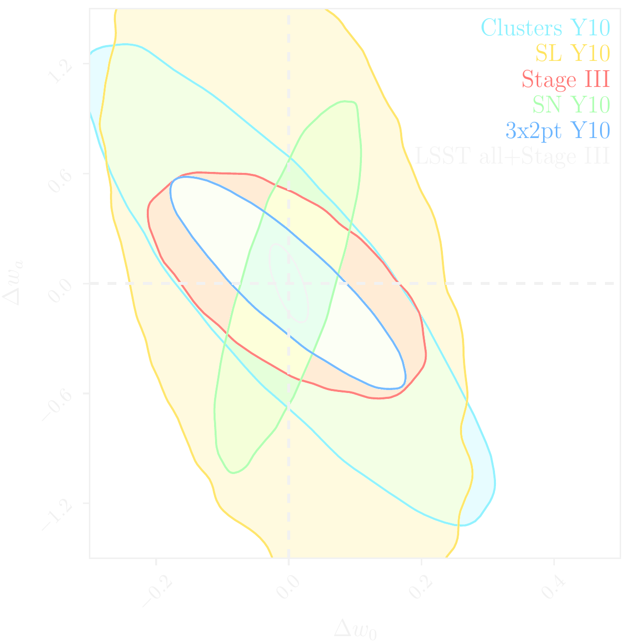
$\Longrightarrow$ Dire need for novel analysis techniques to fully realize the potential of modern surveys.
A few illustrations
Bosch et al. 2017
Jeffrey, Lanusse, et al. 2020
Cheng et al. 2020
- Galaxies are no longer blobs.
- Signals are no longer Gaussian.
- Cosmological likelihoods are no longer tractable.
$\Longrightarrow$ This is the end of the analytic era...
The Deep Learning Explosion in Astrophysics
astro-ph abstracts mentioning Deep Learning, CNN, or Neural
Networks
Review of the impact of Deep Learning in Galaxy Survey Science
https://ml4astro.github.io/dawes-review
Selected examples of Deep Learning in Astrophysics
- Classifying objects
- Inferring object properties
- Self-supervised Representation
Learning
- Solve inverse problems
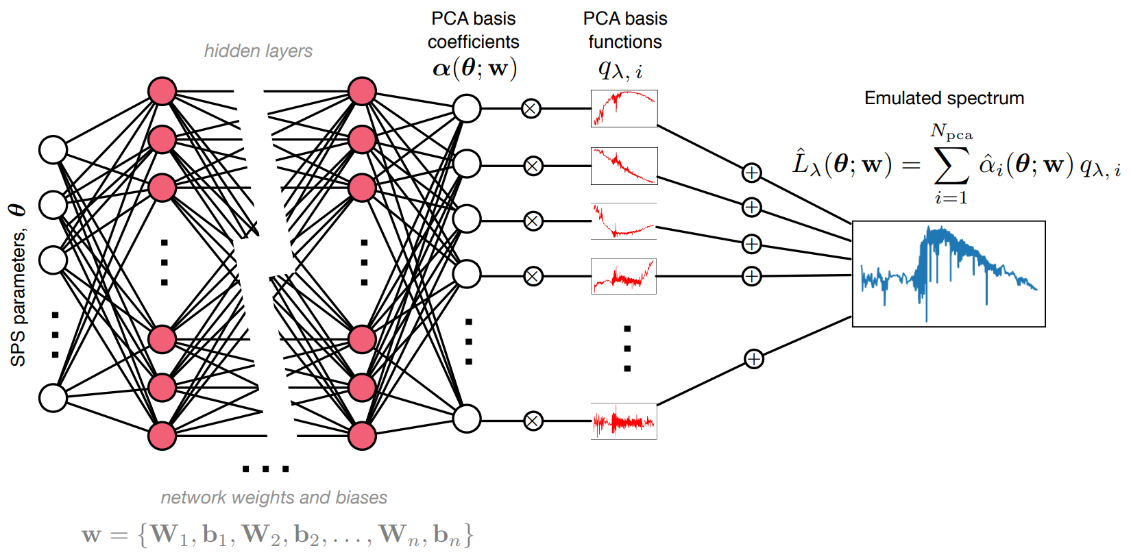
- Emulate costly physical models
- Accelerating numerical simulations
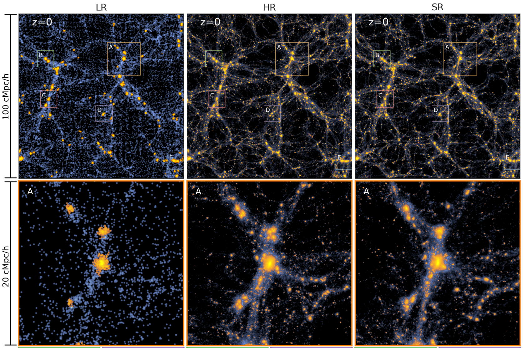
AI-assisted super-resolution cosmological simulations, Li et al. 2021- Enabling Simulation-Based Inference
![]()
![]()
![]()
![]()
![]()
![]()
![]()
- Enabling Simulation-Based Inference
Learning objectives for this lecture
Deep Learning does not create new information, but
allows you to manipulate existing knowledge to answer new questions.
By the end of this lecture you should understand:
- how to interpret neural networks from a Bayesian perspective
- how to apply deep learning to perform Simulation-Based Inference
- how to optimally extract cosmological information from surveys
- how to estimate cosmological posterior without analytic likelihoods
- how to apply deep learning to solve Inverse Problems
- how to learn non-gaussian signal priors
- how to solve inverse problems with explicit likelihoods
A (very) Brief Introduction to Neural Architectures
What is a neural network?
Simplest architecture: Multilayer Perceptron (MLP)
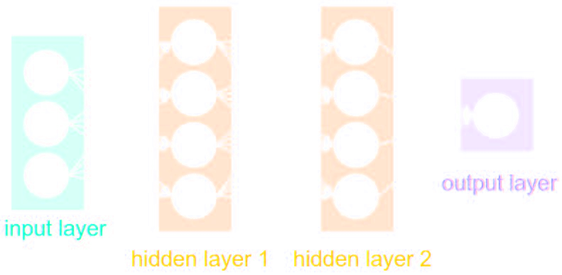
- Series of Dense a.k.a Fully connected layers:
$$ h = \sigma(W x + b)$$
where:
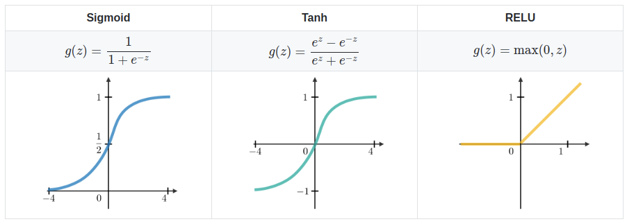
- $\sigma$ is the activation function (e.g. ReLU, Sigmoid, etc.)
- $W$ is a multiplicative weight matrix
- $b$ is an additive bias parameter
- This defines a parametric non-linear function $f_\theta(x)$
- MLPs are universal function approximators
Nota bene: only asymptotically true!
How do you use it to approximate functions?
- Assume a loss function that should be small for good approximations on a training set of data points $(x_i, y_i)$ $$ \mathcal{L} = \sum_{i} ( y_i - f_\theta(x_i))^2 $$
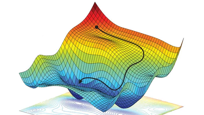
- Optimize the parameters $\theta$ to minimize the loss function by gradient descent $$ \theta_{t+1} = \theta_t - \eta \nabla_\theta \mathcal{L} $$
Different neural architectures for different types of data
Performance can be improved for particular types of data by making use of inductive biases
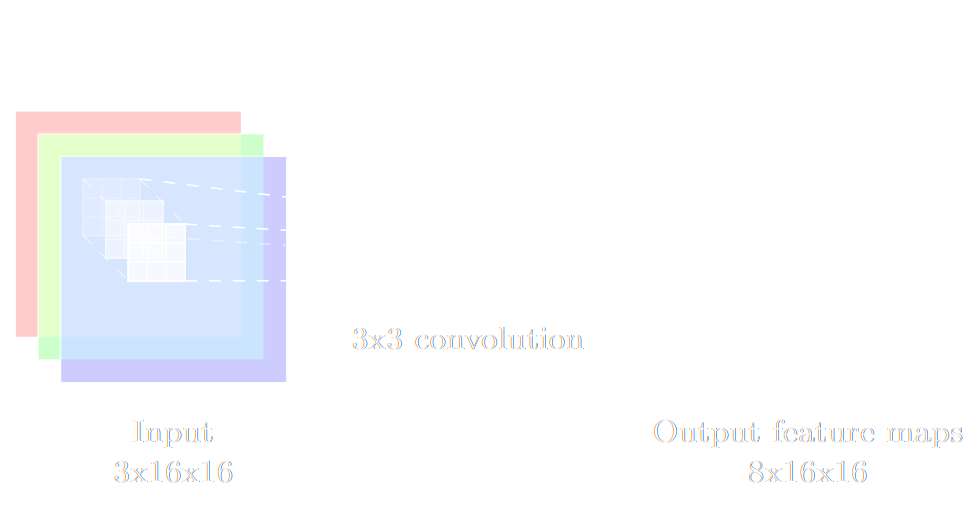 $$ h = \sigma(W \ast x + b)$$

- Image -> Convolutional Networks
- Convolutional layers are translation invariant
- Pixel topology is incorporated by construction
- Time Series -> Recurrent Networks
- Temporal information and variable length is incorporated by construction
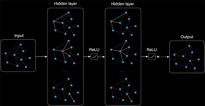
- Graph-stuctured data -> Graph Neural Networks
- Graph topology is incorporated by construction
- Can be seen as generalisation of convolutional networks
$\Longrightarrow$Complete architectures can be compositions of these layers (and others).
takeways
- Depending on the data, different architectures will benefit from different inductive biases.
- In 2023, you can assume that there exists a
neural architecture that can achieve near optimal performance on your data.
Pro tips:- Don't try to reinvent your own architecture, use an existing state of the art one! (e.g. ResNet)
- Most neural network libraries already have most common architectures implemented for you
- The particular neural network you use becomes an implementation detail.
$\Longrightarrow$ For most astrophysical problems, even basic architectures are already good enough.
$\Longrightarrow$ In the rest of this talk all neural networks will just be denoted by a parametric function $f_\theta$
Probabilistic Understanding of Deep Learning
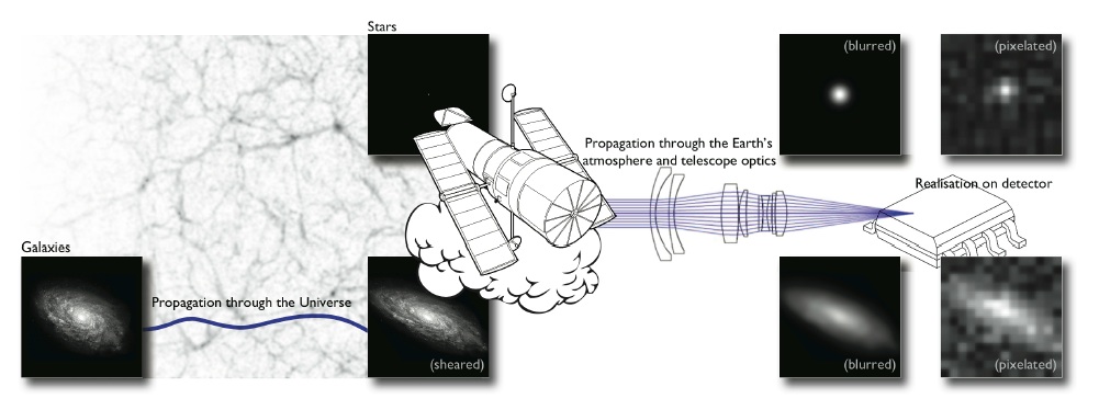
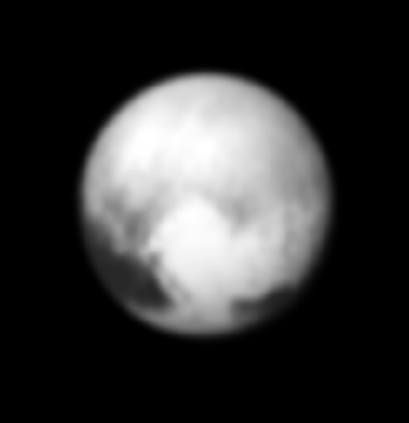
A Motivating Example: Image Deconvolution
$ y = P \ast x + n $
Observed $y$
Ground-Based Telescope
$f_\theta$
some deep Convolutional Neural Network
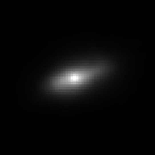
Unknown $x$
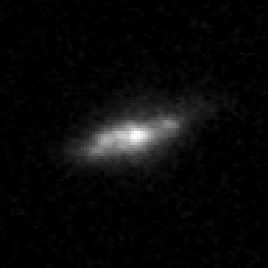
Hubble Space Telescope
- A standard approach would be to train a neural network $f_\theta$ to estimate $x$ given $y$.
- Step I: Assemble from data or simulations a training set of images $$\mathcal{D} = \{(x_0, y_0), (x_1, y_1), \ldots, (x_N, y_N) \}$$ $\Longrightarrow$ the dataset contains hardcoded assumptions about PSF $P$ noise $n$, and galaxy morphology $x$.
- Step II: Train the neural network $f_\theta$ under a regression loss of the type: $$ \mathcal{L} = \sum_{i=0}^N \parallel x_i - f_\theta(y_i)\parallel^2 $$
$$ y $$
$$f_\theta$$
 $$f_\theta(y)$$
$$ \mbox{True } x $$
$\Longrightarrow$Why is the network output different from the truth? If it's
not the truth, then what is $f_\theta(y)$?
A neural network will try to answer
the question you ask.
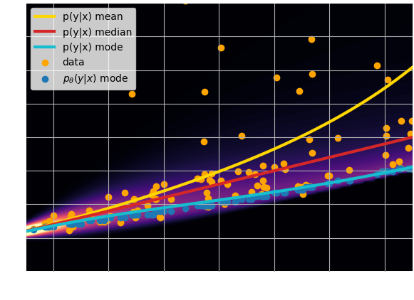
Let's try to understand the neural network output by looking at the loss function
$$ \mathcal{L} = \sum_{(x_i, y_i) \in \mathcal{D}} \parallel x_i - f_\theta(y_i)\parallel^2 \quad \simeq \quad \int \parallel x - f_\theta(y) \parallel^2 \ p(x,y) \ dx dy $$$$\Longrightarrow \int \left[ \int \parallel x -
f_\theta(y) \parallel^2 \ p(x|y) \ dx \right] p(y) dy $$
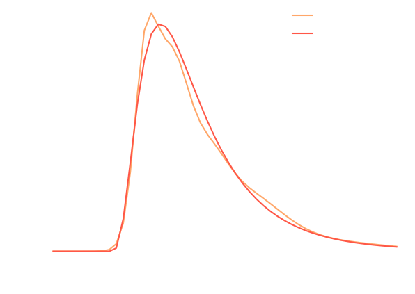
$\mathcal{L}$ minimized when $f_{\theta^\star}(y) = \int x \ p(x|y) \ dx $, i.e.
when $f_{\theta^\star}(x)$ is predicting the mean of $p(x|y)$.
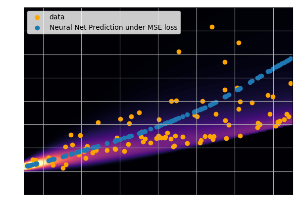
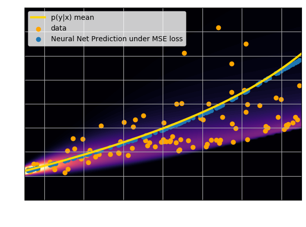
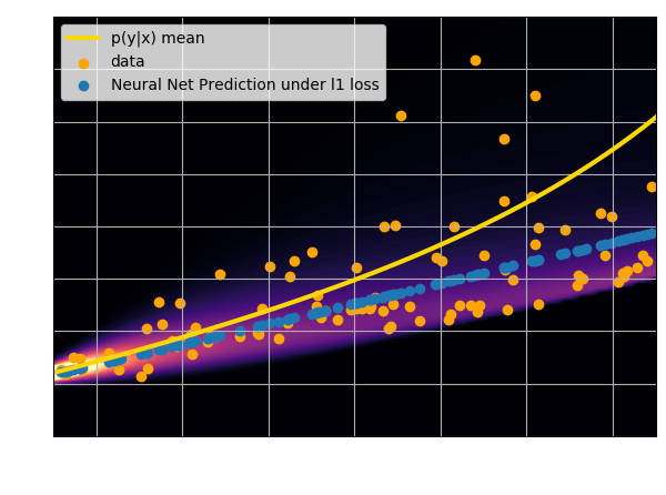
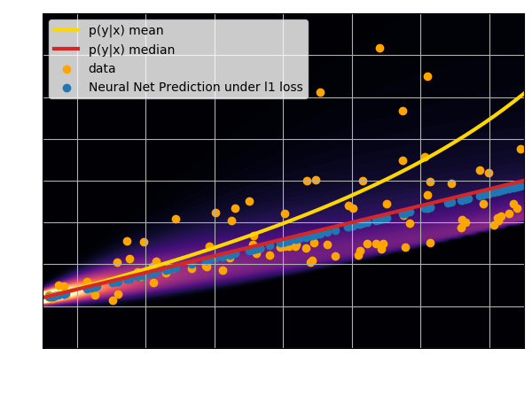
- Using an $\ell_2$ loss learns the mean of the $p(x | y)$
- Using an $\ell_1$ loss learns the median of $p(x|y)$
- In general, training a neural network for
regression doesn't
achieve de mode of the distribution.
Check this blogpost and this notebook to learn how to do that:
Let's take a step back and think as Bayesians
Data $y$
Posterior samples $p(x | y)$
True $x$
- This deconvolution problem is an ill-posed inverse problem $y = A x + n$.
$\Longrightarrow$There is no unique solution, the true answer can never be recovered.
Bayesian point of view
There is a distribution of solutions $p(x|y)$ which can be understood as a Bayesian posterior distribution:
$$ p(x | y) \propto \underbrace{p(y | x)}_{\mbox{likelihood}} \quad
\underbrace{p(x)}_{\mbox{prior}} $$
This brings an interesting question:
- How do I ask a neural network to solve the full Bayesian inference problem?
Step I: We need a parametric conditional density model $q_\phi(x | y)$
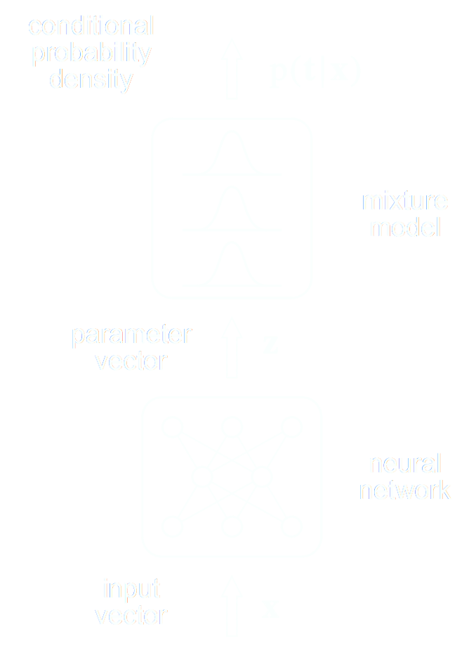
Bishop (1994)
- Mixture Density Networks (MDN) \begin{equation} q_\phi(x | y) = \prod_i \pi^i_\phi(y) \ \mathcal{N}\left(\mu^i_\phi(y), \ \sigma^i_\phi(y) \right) \nonumber \end{equation}
- Flourishing Machine Learning literature on density estimators for higher dimensions.
![]() GLOW, (Kingma & Dhariwal, 2018)
GLOW, (Kingma & Dhariwal, 2018)

Step II: We need a tool to compare distributions
 The Kullback-Leibler divergence:
$$ D_{KL}(p||q) = \mathbb{E}_{x \sim p(x)} \left[ \log \frac{p(x)}{q(x)} \right] $$
The Kullback-Leibler divergence:
$$ D_{KL}(p||q) = \mathbb{E}_{x \sim p(x)} \left[ \log \frac{p(x)}{q(x)} \right] $$
$$D_{KL}(p(x | y) ||q_\phi(x | y)) = \mathbb{E}_{x \sim p(x |y)} \left[ \log \frac{p(x | y)}{q_\phi(x | y)} \right] \geq 0 $$
$$ \leq \mathbb{E}_{y \sim p(y)} \mathbb{E}_{x \sim p(x |y)} \left[ \log \frac{p(x | y)}{q_\phi(x | y)} \right] $$
$$ \leq \boxed{ \mathbb{E}_{(y,x) \sim p(y, x)} \left[ - \log q_\phi(x | y) \right] } + cst $$
$\Longrightarrow$ Minimizing the Negative Log Likelihood (NLL) over the joint distribution $p(x, y)$
leads to minimizing the KL divergence between the model posterior $q_{\phi}(x|y)$ and true posterior $p(x | y)$.
Step III: Assembling the training set $\mathcal{D} = \left\{ (x_i, y_i) \sim p(x, y) \right\} $
- 1. Sample $x_i$ from $p(x)$
![]()
- 2. Sample $y_i$ from $p(y|x_i)$
![]()
Sampling from the joint distribution can be expressed as:
$$ (x, y) \sim p(x, y) = \underbrace{p(y | x)}_{\mathrm{likelihood}} \ \underbrace{p(x)}_{\mathrm{prior}} $$
A few comments:
- Priors AND likelihoods are hardcoded in the training set.
- If your data is based on simulations you control both
- If your data is observational, be very careful and cognizant of the fact that selection effects in your dataset translate as implicit priors.
Summarizing the Probabilistic Deep Learning Recipe
- Express the output of the model as a distribution, not a point estimate $$ q_\phi(x | y) $$
- Assemble a training set that encodes your prior on the problem $$ \mathcal{D} = \left\{ (x_i, y_i) \sim p(x, y) = p(y|x) p(x) \right\} $$
- Optimize for the Negative Log Likelihood $$\mathcal{L} = - \log q_\phi(x|y) $$
- Profit!
- Interpretable network outputs (i.e. I know mathematically what my network is trying to approximate)
- Uncertainty quantification (i.e. Bayesian Inference)
takeaways
- Unless the relationship between input and outputs of your problem is purely deterministic (e.g. power spectrum emulator), you should think under a probabilistic model to understand what the network is doing.
- Conditional density estimation is superior to point estimates
- Provides uncertainty quantification
- Even if a point estimate is desired, gives access to the Maximum a Posteriori
- We have learned how to pose a Deep Learning question:
- A loss function $\mathcal{L}$ and training set $\mathcal{D}$
$\Longrightarrow$ Mathematically defines the solution you are trying to get. - An appropriate architecture $q_\phi$
$\Longrightarrow$ This is the tool you are using to solve the problem.
- A loss function $\mathcal{L}$ and training set $\mathcal{D}$
If you want to try it!
Checkout this notebook: this notebook.
Your goal:
Building a regression model with a Mean Squared Error loss in JAX/FlaxExample of Application:
Simulation-Based Inference
The limits of traditional cosmological inference
HSC cosmic shear power spectrum
HSC Y1 constraints on $(S_8, \Omega_m)$
(Hikage et al. 2018)
- Measure the ellipticity $\epsilon = \epsilon_i + \gamma$ of all galaxies
$\Longrightarrow$ Noisy tracer of the weak lensing shear $\gamma$ - Compute summary statistics based on 2pt functions,
e.g. the power spectrum - Run an MCMC to recover a posterior on model parameters, using an analytic likelihood $$ p(\theta | x ) \propto \underbrace{p(x | \theta)}_{\mathrm{likelihood}} \ \underbrace{p(\theta)}_{\mathrm{prior}}$$
Main limitation: the need for an explicit likelihood
We can only compute from theory the likelihood for simple summary statistics and on large scales
$\Longrightarrow$ We are dismissing a significant fraction of the information!
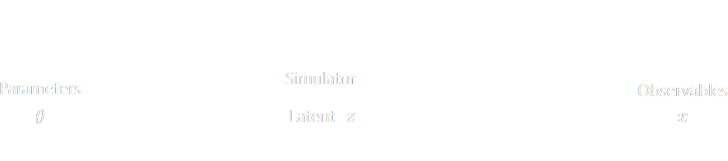
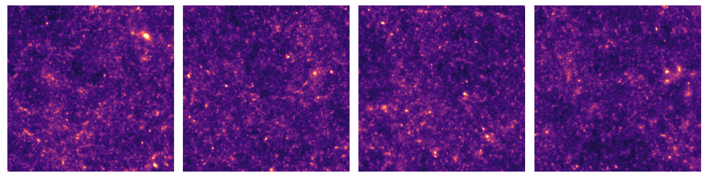
Full-Field Simulation-Based Inference
- Instead of trying to analytically evaluate the likelihood of
sub-optimal summary statistics, let us build a forward model of the full observables.
$\Longrightarrow$ The simulator becomes the physical model. - Each component of the model is now tractable, but at the cost of a large number of latent variables.
Benefits of a forward modeling approach
- Fully exploits the information content of the data (aka "full field inference").
- Easy to incorporate systematic effects.
- Easy to combine multiple cosmological probes by joint simulations.
...so why is this not mainstream?
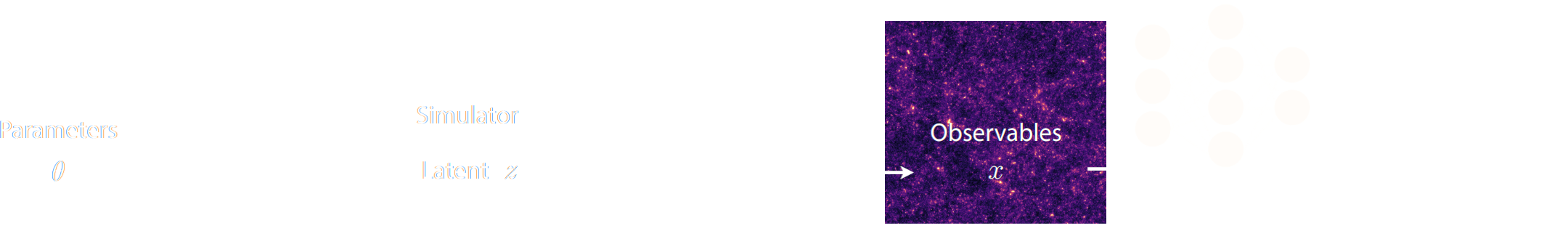
The Challenge of Simulation-Based Inference
$$ p(x|\theta) = \int p(x, z | \theta) dz = \int p(x | z, \theta) p(z | \theta) dz $$
Where $z$ are stochastic latent variables of the simulator.
$\Longrightarrow$ This marginal likelihood is intractable!
$\Longrightarrow$ This marginal likelihood is intractable!
Black-box Simulators Define Implicit Distributions
- A black-box simulator defines $p(x | \theta)$ as an implicit distribution, you can sample from it but you cannot evaluate it.
- Key Idea: Use a parametric distribution model $\mathbb{P}_\varphi$ to approximate the implicit distribution $\mathbb{P}$.

True $\mathbb{P}$

Samples $x_i \sim \mathbb{P}$

Model $\mathbb{P}_\varphi$
Deep Learning Approaches to Implicit Inference
A two-steps approach to Implicit Inference
- Automatically learn an optimal low-dimensional summary statistic $$y = f_\varphi(x) $$
- Use Neural Density Estimation to either:
- build an estimate $p_\phi$ of the likelihood function $p(y \ | \ \theta)$ (Neural Likelihood Estimation)
- build an estimate $p_\phi$ of the posterior distribution $p(\theta \ | \ y)$ (Neural Posterior Estimation)
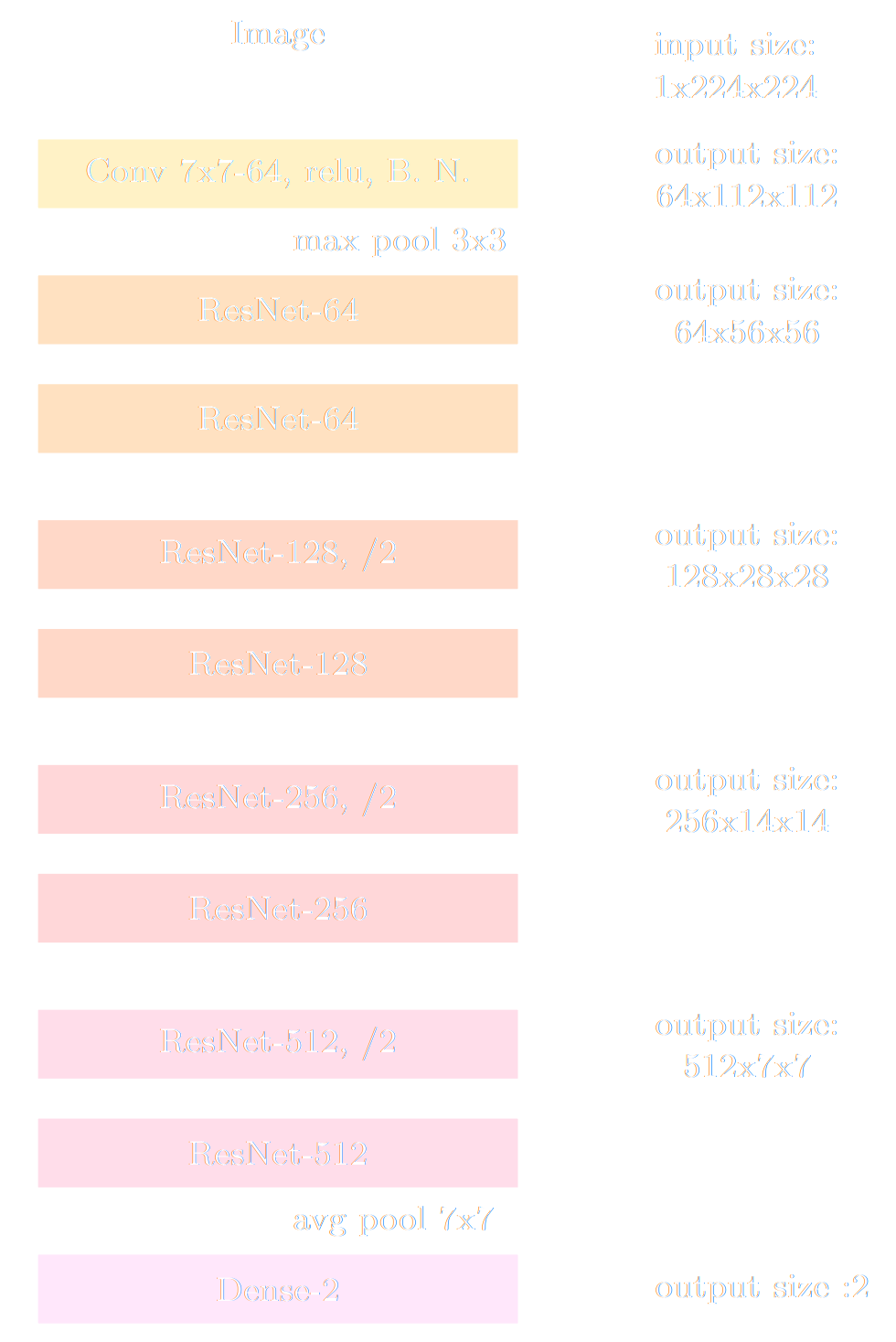
Automated Summary Statistics Extraction
- Introduce a parametric function $f_\varphi$ to reduce the dimensionality of the data while preserving information.
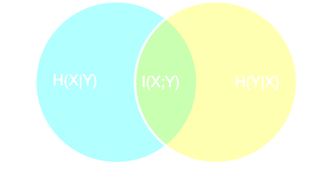
Information-based loss functions
- Summary statistics $y$ is sufficient for $\theta$ if $$ I(Y; \Theta) = I(X; \Theta) \Leftrightarrow p(\theta | x ) = p(\theta | y) $$
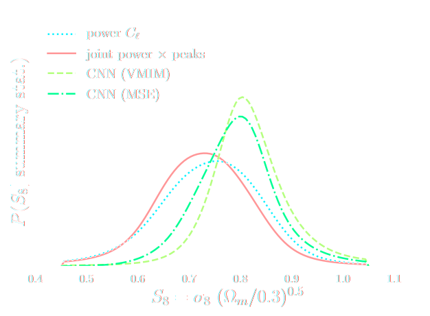
- Variational Mutual Information Maximization
$$ \mathcal{L} \ = \ \mathbb{E}_{x, \theta} [ \log q_\phi(\theta | f_\varphi(x)) ] \leq I(Y; \Theta) $$
Jeffrey, Alsing, Lanusse (2021)

Unrolling the Probabilistic Learning Recipe
- I assume a forward model of the observations: \begin{equation} p( x ) = p(x | \theta) \ p(\theta) \nonumber \end{equation} All I ask is the ability to sample from the model, to obtain $\mathcal{D} = \{x_i, \theta_i \}_{i\in \mathbb{N}}$
- I am going to assume $q_\phi(\theta | x)$ a parametric conditional density
- Optimize the parameters $\phi$ of $q_{\phi}$ according to \begin{equation} \min\limits_{\phi} \sum\limits_{i} - \log q_{\phi}(\theta_i | x_i) \nonumber \end{equation} In the limit of large number of samples and sufficient flexibility \begin{equation} \boxed{q_{\phi^\ast}(\theta | x) \approx p(\theta | x)} \nonumber \end{equation}
$\Longrightarrow$ One can asymptotically recover the posterior by
optimizing a parametric estimator over
the Bayesian joint distribution
the Bayesian joint distribution
$\Longrightarrow$ One can asymptotically recover the posterior by
optimizing a Deep Neural Network over
a simulated training set.
a simulated training set.
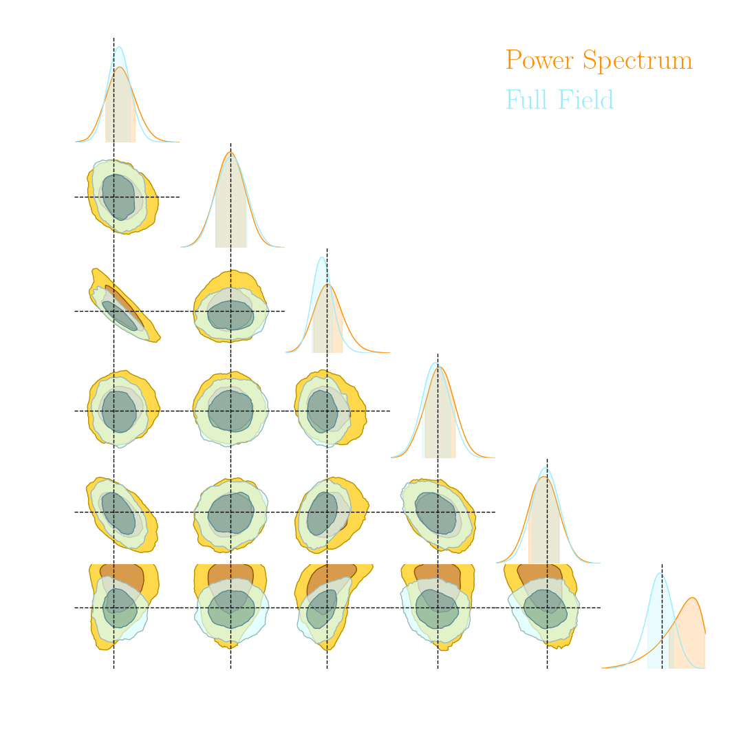
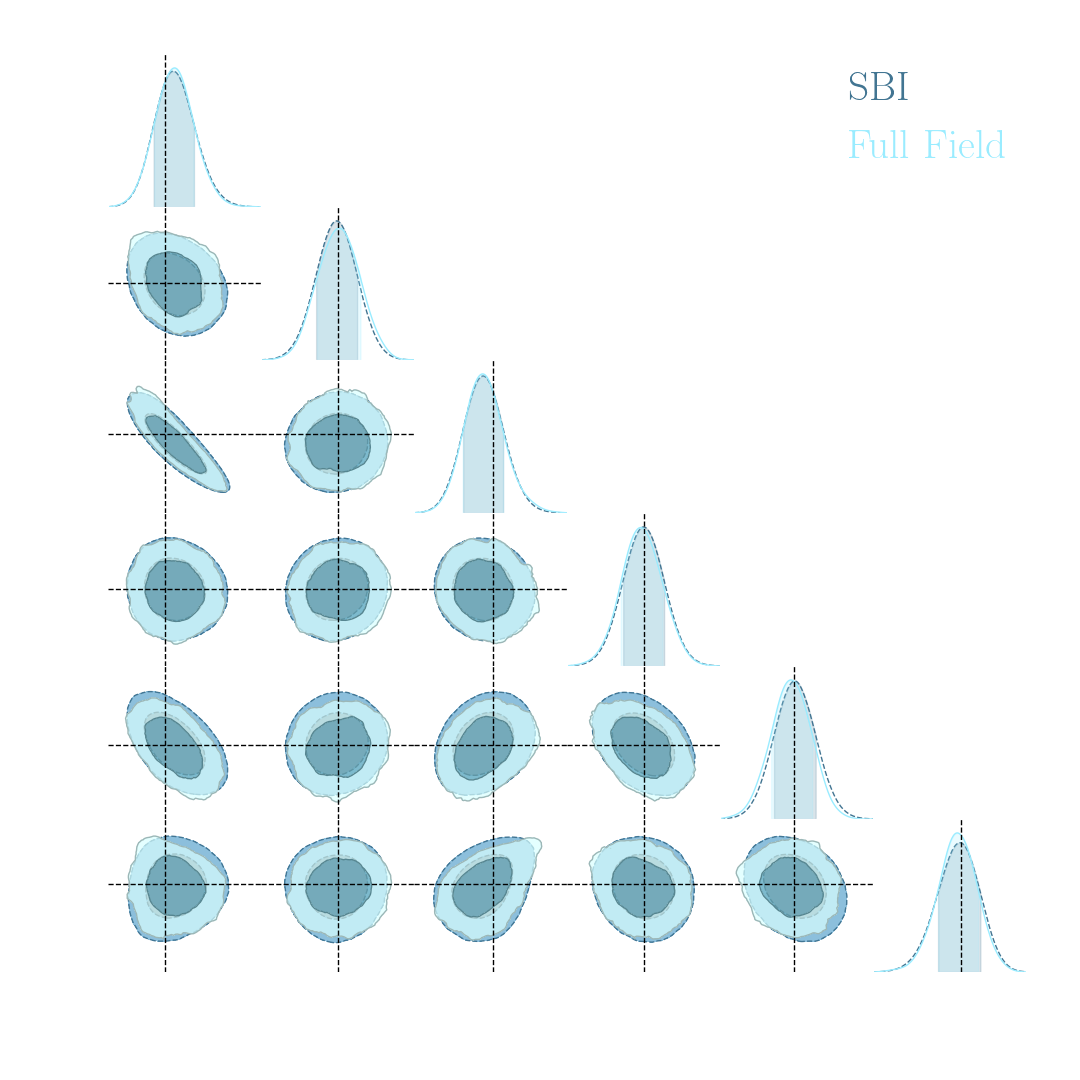
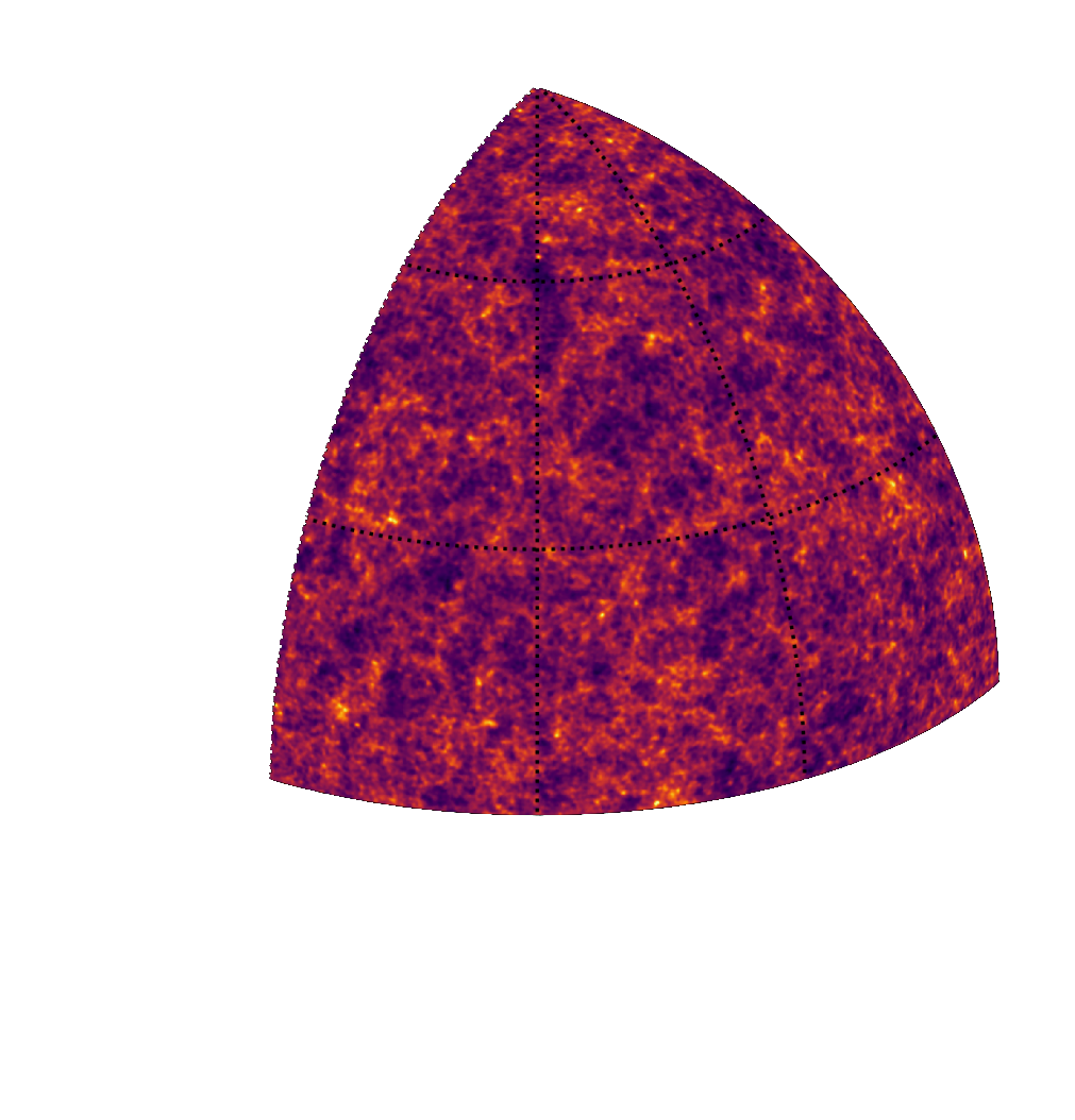
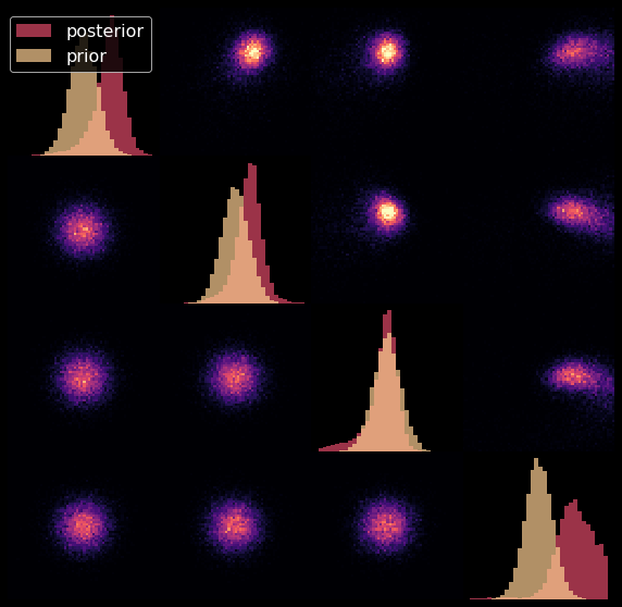
Illustration on log-normal lensing simulations

DifferentiableUniverseInitiative/sbi_lens
JAX-based log-normal lensing simulation package
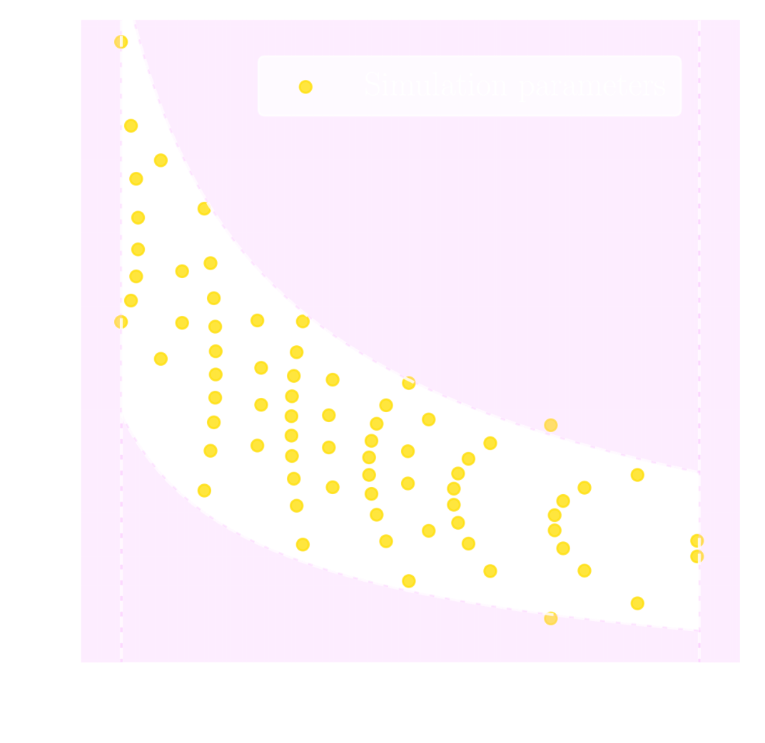
- 10x10 deg$^2$ maps at LSST Y10 quality, conditioning the log-normal shift parameter on $(\Omega_m, \sigma_8, w_0)$
- Infer full-field posterior on cosmology:
- explicitly using an Hamiltonian-Monte Carlo (NUTS) sampler
- implicitly using a learned summary statistics and conditional density estimation.
A variety of algorithms
Lueckmann, Boelts, Greenberg, Gonçalves, Macke (2021) 
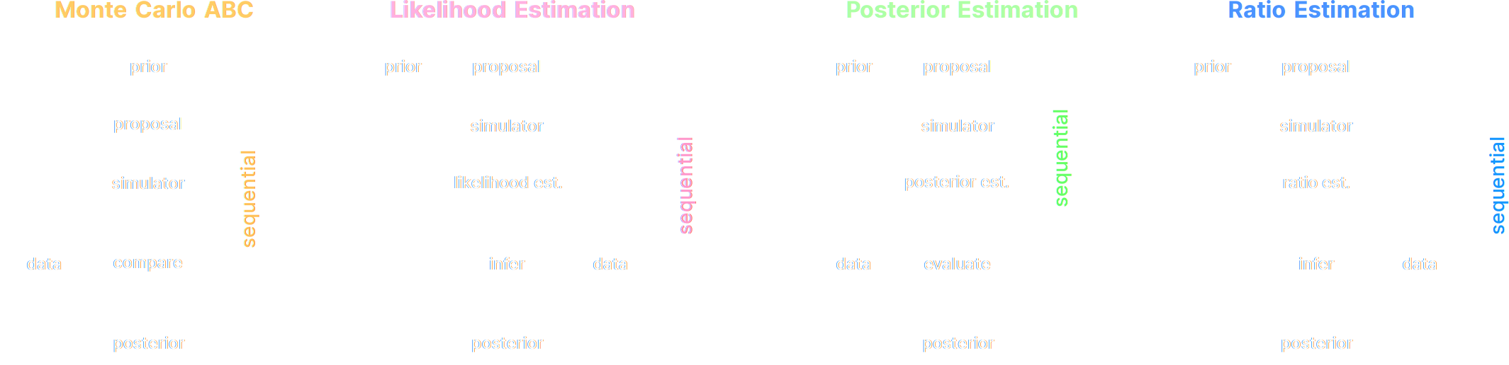
A few important points:
- Amortized inference methods, which estimate $p(\theta | x)$, can greatly speed up posterior estimation once trained.
- Sequential Neural Posterior/Likelihood Estimation methods can actively sample simulations needed to refine the inference.
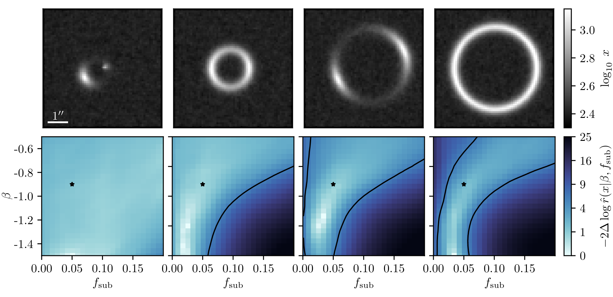
Example of application: Constraining Dark Matter Substructures
Brehmer, Mishra-Sharma, Hermans, Louppe, Cranmer (2019) 

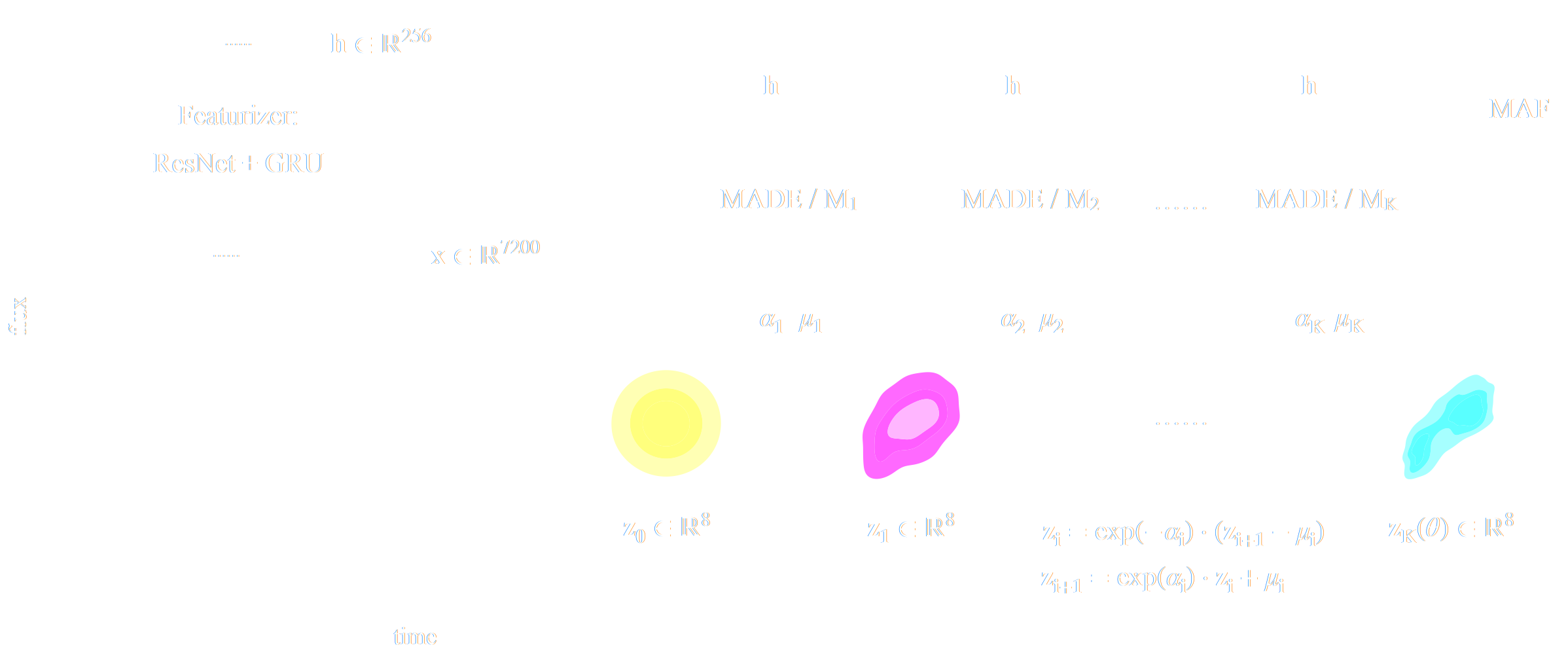
Example of application: Infering Microlensing Event Parameters
Zhang, Bloom, Gaudi, Lanusse, Lam, Lu (2021) 
Example of application: Likelihood-Free parameter inference with DES SV
Jeffrey, Alsing, Lanusse (2021)
Suite of N-body + raytracing simulations: $\mathcal{D}$
Main takeaways
- This approach automatizes cosmological inference
- Turns the summary extraction and inference problems into an optimization problems
- If neural networks fail, inference will be sub-optimal but not necessarily biased.
- Some resources and links:
- Review on Simulation-Based Inference: Cranmer, Brehmer, Louppe (2020)
- Recent full $w$CDM Likelihood-Free Inference constraints on DES Y3: Fluri, Kacprzak, Lucchi, Schneider, Refregier, Hofmann (2022)
- Simulation Based Inference packages: sbi, pydelfy, Information Maximizing Neural Networks
Deep Generative Modeling
What is generative modeling?
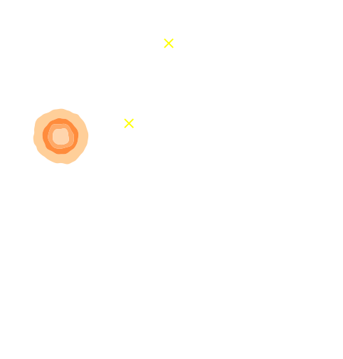
- The goal of generative modeling is to learn an implicit distribution $\mathbb{P}$ from which the training set $X = \{x_0, x_1, \ldots, x_n \}$ is drawn.
- Usually, this means building a parametric model $\mathbb{P}_\theta$ that tries to be close to $\mathbb{P}$.
True $\mathbb{P}$
Samples $x_i \sim \mathbb{P}$
Model $\mathbb{P}_\theta$
- Once trained, you can typically sample from $\mathbb{P}_\theta$ and/or evaluate the likelihood $p_\theta(x)$.
Why isn't it easy?
- The curse of dimensionality put all points far apart in high dimension


Distance between pairs of points drawn from a Gaussian distribution.
- Classical methods for estimating probability densities, i.e. Kernel Density Estimation (KDE) start to fail in high dimension because of all the gaps
The evolution of generative models
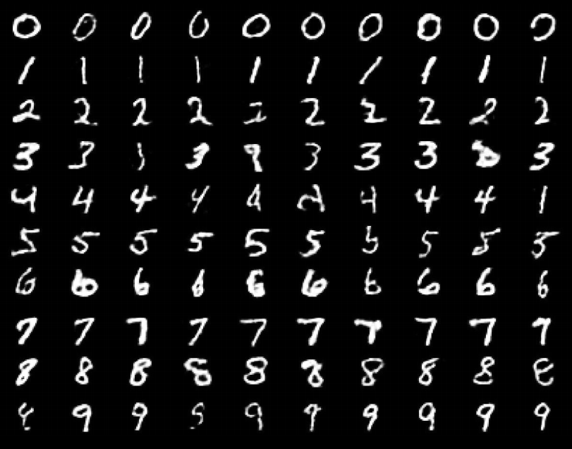
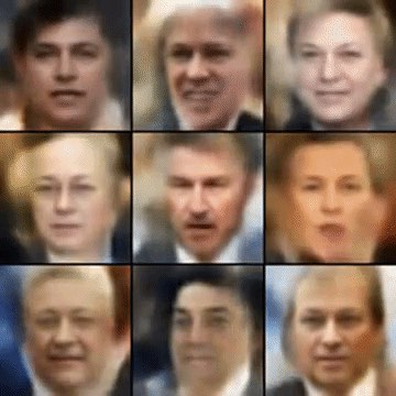
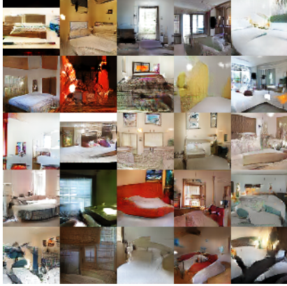
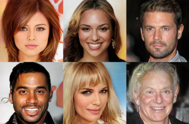
- Deep Belief Network
(Hinton et al. 2006) - Variational AutoEncoder
(Kingma & Welling 2014) - Generative Adversarial Network
(Goodfellow et al. 2014) - Wasserstein GAN
(Arjovsky et al. 2017) - Midjourney v5 Guided Diffusion (2023)
A brief survey of Generative Models Families

- Latent Variable Models:
Assume the following form for the model disribution: $$ x = f_\theta(z) \qquad \mbox{with} \qquad z \sim p(z)$$ This is the case of Generative Adversarial Networks, Variational Auto-Encoders, Normalizing Flows. - Auto-Regressive Models:
Assume an autoregressive decomposition of the signal into products of 1D conditional distributions: $$ p_\theta(x) = p_\theta(x_0) p_\theta(x_1 | x_0) \ldots p_\theta(x_n | x_{n-1}, \ldots x_{0}) $$ This is the case of PixelCNN, GPT-3 - Diffusion Models:
Target distribution generated by a reverse noise diffusion process controled by a Stochastic Differential Equation (SDE).
The Variational Auto-Encoder
- We assume a prior distribution $p(z)$ for the latent variable, and a likelihood $p_\theta(x |z)$ defined by a neural network.
Typically $p_\theta(x|z) = \mathcal{N}(x; f_\theta(x), \sigma^2)$ - Training the generative model amounts to finding $\theta_\star$ that
maximizes the marginal likelihood of the model:
$$p_\theta(x) = \int \mathcal{N}(x; f_\theta(z), \sigma^2) \ p(z) \ dz$$
$\Longrightarrow$ This is generally intractable
- In a VAE, efficient training of parameter $\theta$ is made possible by Amortized Variational Inference.
Auto-Encoding Variational Bayes (Kingma & Welling, 2014)
- We introduce a parametric distribution $q_\phi(z | x)$ which aims to model the posterior $p(z | x)$. We want to minimize $\mathbb{D}_{KL}\left( q_\phi(z | x) \parallel p(z | x) \right)$
- Working out the KL divergence between these two distributions leads to: $$\log p_\theta(x) \quad \geq \quad - \mathbb{D}_{KL}\left( q_\phi(z | x) \parallel p(z) \right) \quad + \quad \mathbb{E}_{z \sim q_{\phi}(. | x)} \left[ \log p_\theta(x | z) \right]$$ $\Longrightarrow$ This is the Evidence Lower-Bound, which is differentiable with respect to $\theta$ and $\phi$.
The famous Variational Auto-Encoder
$$\log p_\theta(x) \geq - \underbrace{\mathbb{D}_{KL}\left( q_\phi(z | x) \parallel p(z) \right)}_{\mbox{code regularization}} + \underbrace{\mathbb{E}_{z \sim q_{\phi}(. | x)} \left[ \log p_\theta(x | z) \right]}_{\mbox{reconstruction error}} $$
Normalizing Flows
Still a latent variable model, except the mapping $f_\theta$ is made to be bijective.
Dinh et al. 2016
Normalizing Flows
- Assumes a bijective mapping between data space $x$ and latent space $z$ with prior $p(z)$: $$ z = f_{\theta} ( x ) \qquad \mbox{and} \qquad x = f^{-1}_{\theta}(z)$$
- Admits an explicit marginal likelihood: $$ \log p_\theta(x) = \log p(z) + \log \left| \frac{\partial f_\theta}{\partial x} \right|(x) $$
$\Longrightarrow$ The challenge is in designing mappings $f_\theta$ that are both:
easy to invert, easy to compute the jacobian of.
One example of NF: RealNVP
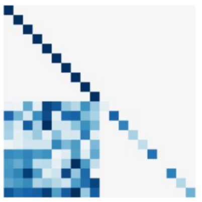
Jacobian of an affine coupling layer
In a standard affine RealNVP, one Flow layer is defined as:
$$ \begin{matrix} y_{1\ldots d} &=& x_{1 \ldots d} \\
y_{d+1\ldots N} &=& x_{d+1 \ldots N} ⊙ \sigma_\theta(x_{1 \ldots d}) + \mu_\theta(x_{1 \ldots d})
\end{matrix} $$
where $\sigma_\theta$ and $\mu_\theta$ are unconstrained neural networks.
We will call this layer an affine coupling.
We will call this layer an affine coupling.
$\Longrightarrow$ This structure has the advantage that the Jacobian of this layer will be lower triangular which makes computing its determinant easy.
Not all generative models are created equal
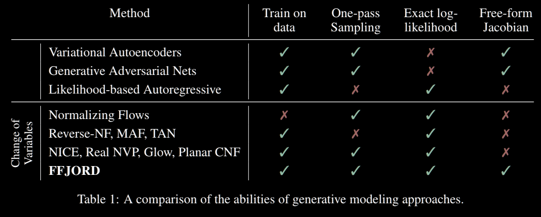
Grathwohl et al. 2018
- Of particular interest are models with an explicit $\log p(x)$ (not the case of VAEs, GANs, Denoising Diffusion Models).
Why are these generative models useful?
Implicit distributions are everywhere!
Case I: Examples from data, no accurate physical model
![]()
Mandelbaum et al. 2014
Case II: Physical model only available as a simulator
![]()
Osato et al. 2020
$\Longrightarrow$ Generative models will enable Bayesian
inference in cases where
implicit distributions are involved, by providing a tractable $p_\theta(x)$.
Your Turn!
We will be using this notebook to implement a Normalizing Flow in JAX+Flax+TensorFlow Probability
Example of application:
Solving Inverse Problems
Back to our Motivating Example
Hubble Space Telescope
some deep neural network
Simulated Ground-Based Telescope
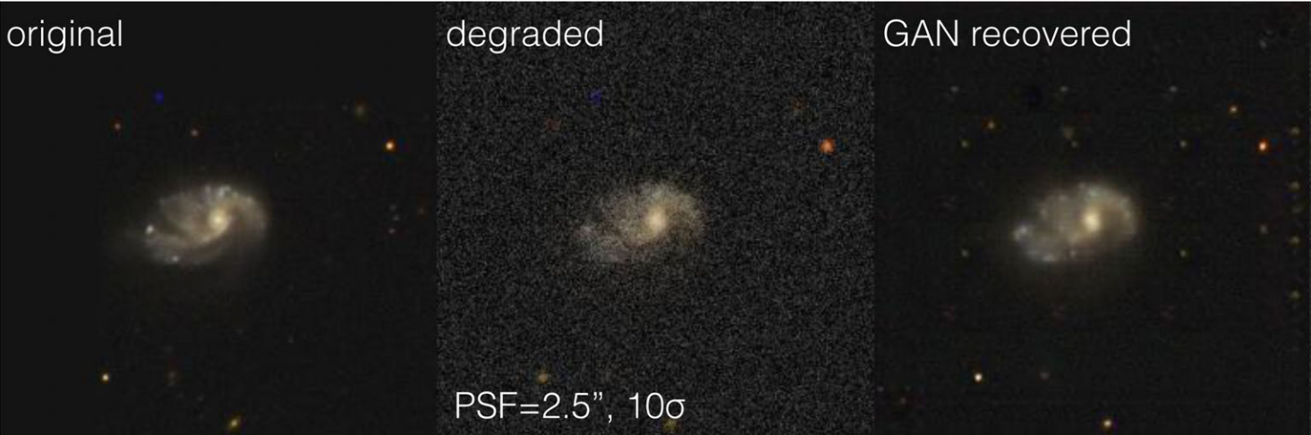
The issue with generic black box deep learning inference
- No explicit control of noise, PSF, depth.
- Unless covered by the training data, the result becomes unpredictable.
- No guarantees some physical properties are preserved
$\Longrightarrow$ In this case, the flux of the deconvolved object - Robust quantification of uncertainties is extremely difficult.
Example: GalaxyGAN (Schawinski et al. 2017)
Linear inverse problems
$\boxed{y = \mathbf{A}x + n}$$\mathbf{A}$ is known and encodes our physical understanding of the problem.
$\Longrightarrow$ When non-invertible or ill-conditioned, the inverse problem is ill-posed with no unique solution $x$
 Deconvolution
 Inpainting
 Denoising
A Bayesian view of the problem
$\boxed{y = \mathbf{A}x + n}$
$$ p(x | y) \propto p(y | x) \ p(x) $$
- $p(y | x)$ is the data likelihood, which contains the
physics
- $p(x)$ is our prior knowledge on the solution.
With these concepts in hand, we want to estimate the Maximum A Posteriori solution:
$$\hat{x} = \arg\max\limits_x \ \log p(y \ | \ x) + \log p(x)$$
For instance, if $n$ is Gaussian, $\hat{x} = \arg\max\limits_x \ - \frac{1}{2} \parallel y - \mathbf{A} x \parallel_{\mathbf{\Sigma}}^2 + \log p(x)$
$$\hat{x} = \arg\max\limits_x \ \log p(y \ | \ x) + \log p(x)$$
For instance, if $n$ is Gaussian, $\hat{x} = \arg\max\limits_x \ - \frac{1}{2} \parallel y - \mathbf{A} x \parallel_{\mathbf{\Sigma}}^2 + \log p(x)$
How do you choose the prior ?
Classical examples of signal priors
Sparse
![]()
$$ \log p(x) = \parallel \mathbf{W} x \parallel_1 $$
$$ \log p(x) = \parallel \mathbf{W} x \parallel_1 $$
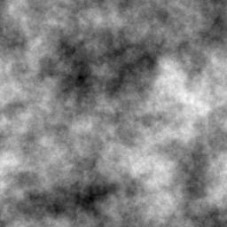
Gaussian
![]() $$ \log p(x) = x^t \mathbf{\Sigma^{-1}} x $$
$$ \log p(x) = x^t \mathbf{\Sigma^{-1}} x $$
 $$ \log p(x) = x^t \mathbf{\Sigma^{-1}} x $$
Total Variation
![]() $$ \log p(x) = \parallel \nabla x \parallel_1 $$
$$ \log p(x) = \parallel \nabla x \parallel_1 $$
But what about this?
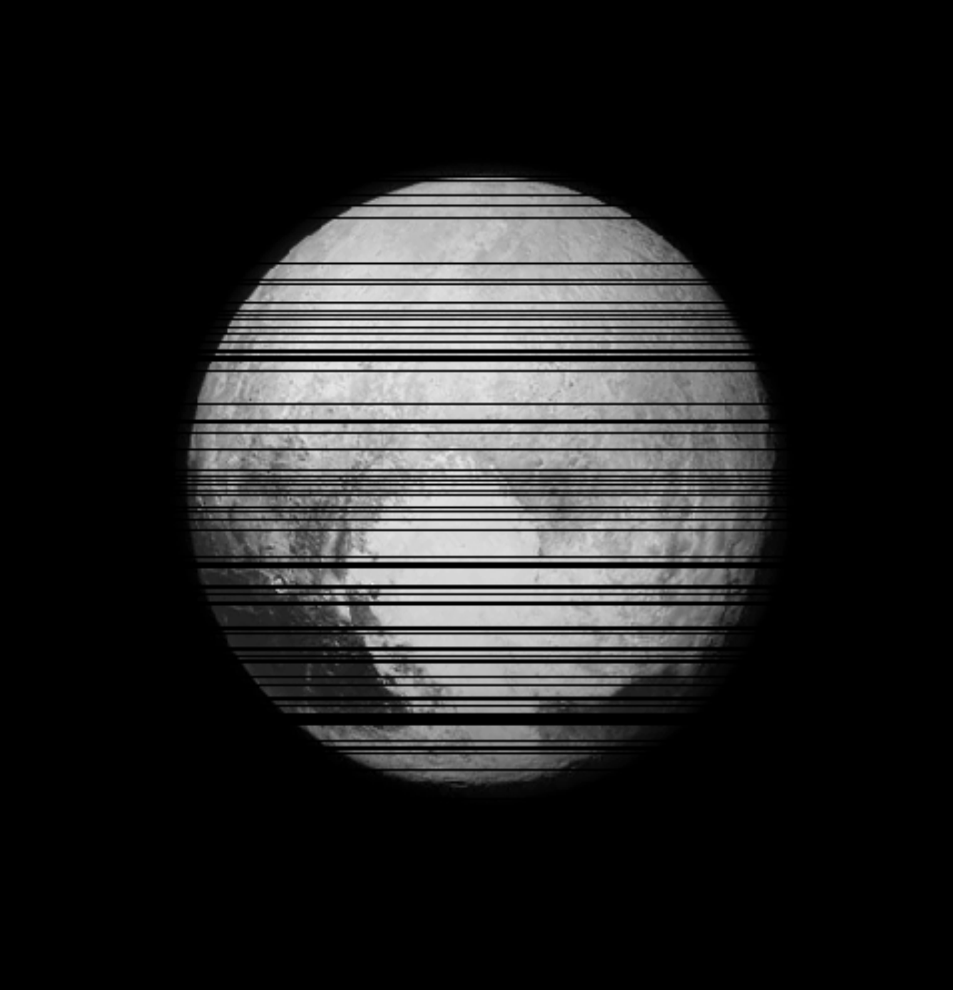
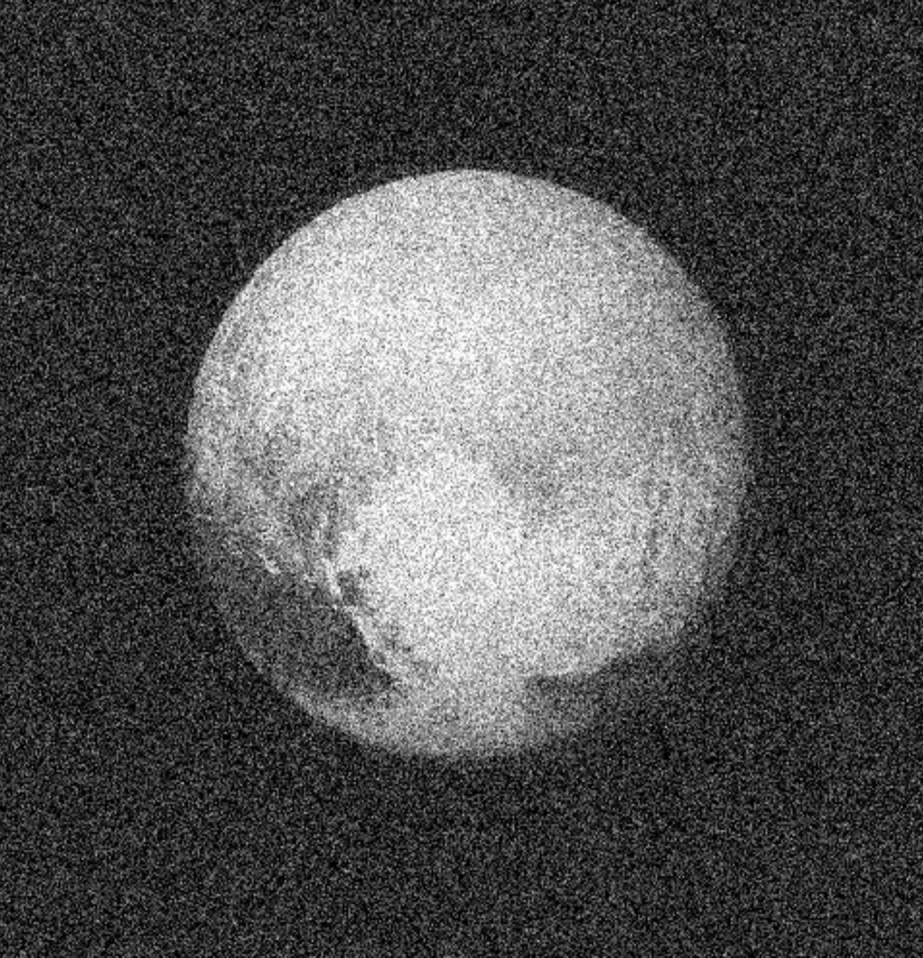
Getting started with Deep Priors: deep denoising example
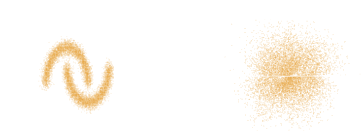
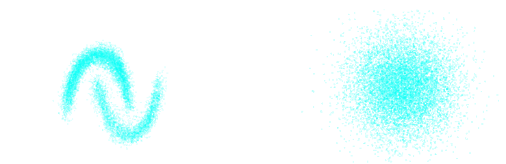
$$ \boxed{{\color{Orchid} y} = {\color{SkyBlue} x} + n} $$
- Let us assume we have access to examples of $ {\color{SkyBlue} x}$ without noise.
- We learn the distribution of noiseless data $\log p_\theta(x)$ from samples using a deep generative model.
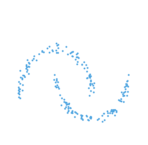
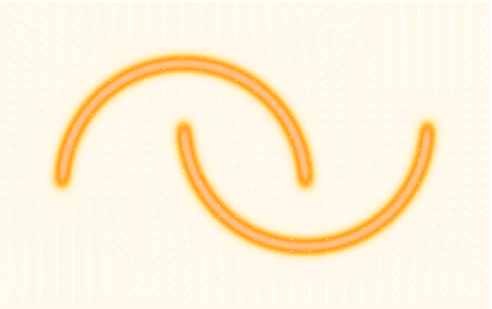
- The solution should lie on the realistic data
manifold, symbolized by the two-moons distribution.
We want to solve for the Maximum A Posterior solution:
$$\arg \max - \frac{1}{2} \parallel {\color{Orchid} y} - {\color{SkyBlue} x} \parallel_2^2 + \log p_\theta({\color{SkyBlue} x})$$ This can be done by gradient descent as long as one has access to the score function $\frac{\color{orange} d \color{orange}\log \color{orange}p\color{orange}(\color{orange}x\color{orange})}{\color{orange} d \color{orange}x}$.
The Scarlet algorithm: deblending as an optimization problem
Melchior et al. 2018
$$ \mathcal{L} = \frac{1}{2} \parallel \mathbf{\Sigma}^{-1/2} (\ Y - P \ast A S \ ) \parallel_2^2 - \sum_{i=1}^K \log p_{\theta}(S_i) + \sum_{i=1}^K g_i(A_i) + \sum_{i=1}^K f_i(S_i)$$
Where for a $K$ component blend:
- $P$ is the convolution with the instrumental response
- $A_i$ are channel-wise galaxy SEDs, $S_i$ are the morphology models
- $\mathbf{\Sigma}$ is the noise covariance
- $\log p_\theta$ is a PixelCNN prior
- $f_i$ and $g_i$ are arbitrary additional non-smooth consraints, e.g. positivity, monotonicity...
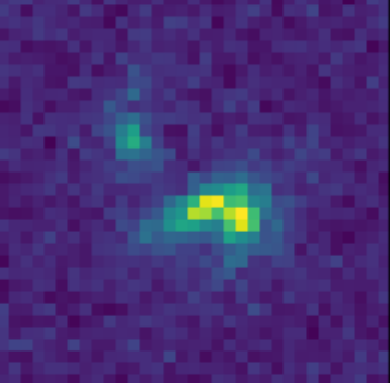
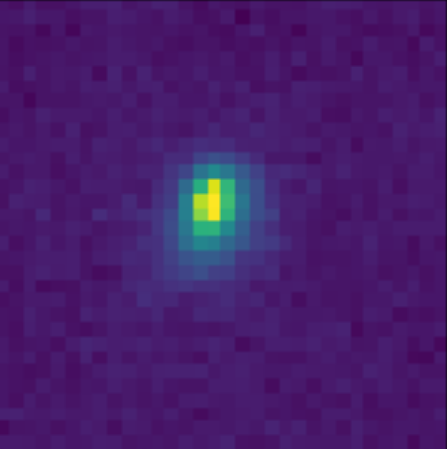
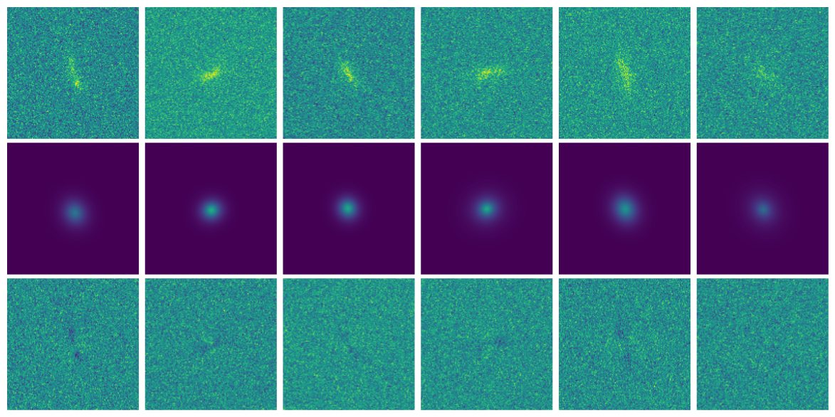
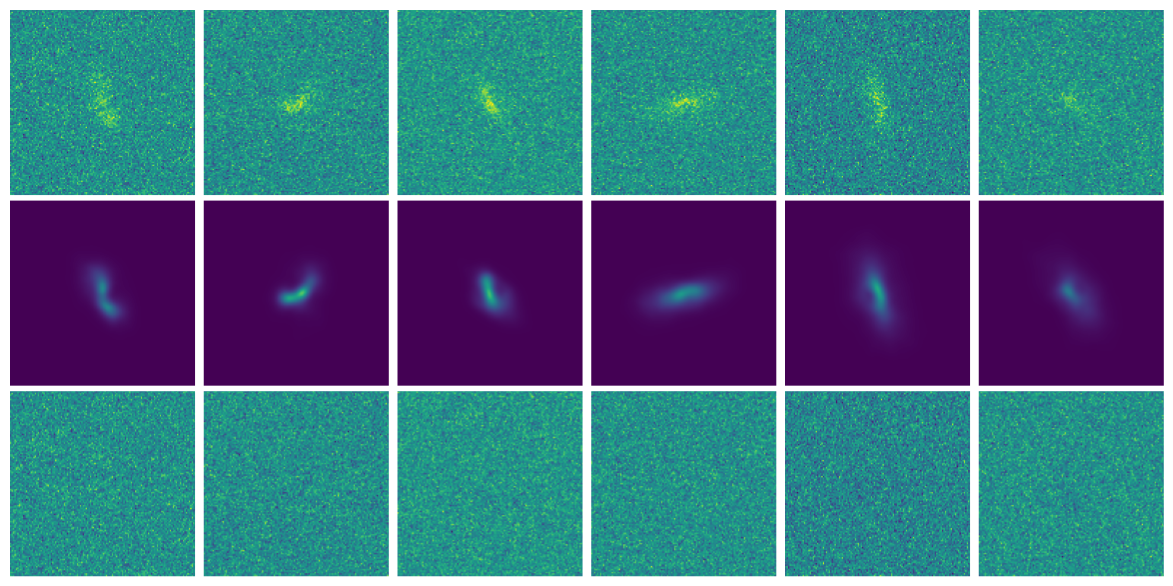
Training the morphology prior
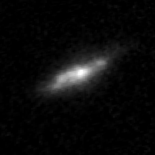
Postage stamps of isolated COSMOS galaxies used for training, at WFIRST resolution and fixed fiducial PSF
isolated galaxy
![]() $\log p_\theta(x) = 3293.7$
$\log p_\theta(x) = 3293.7$
 $\log p_\theta(x) = 3293.7$
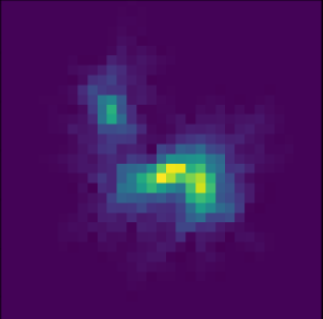
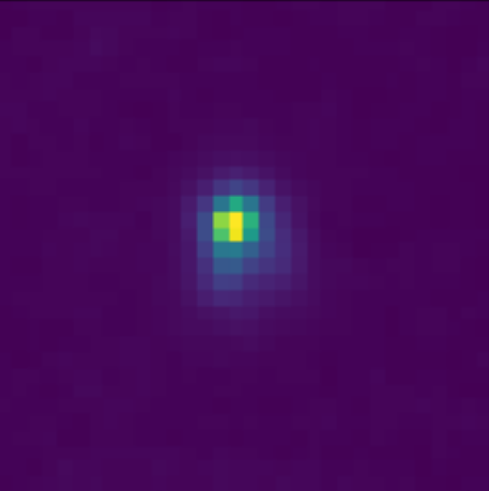
artificial blend
![]() $\log p_\theta(x) = 3100.5 $
$\log p_\theta(x) = 3100.5 $
 $\log p_\theta(x) = 3100.5 $
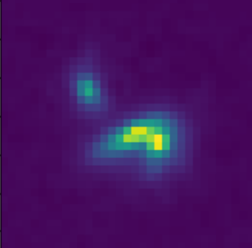
Scarlet in action
Input blend
![]()
Solution
![]()
![]()
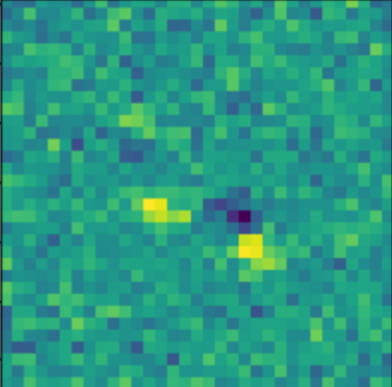
Residuals
![]()
![]()
- Classic priors (monotonicity, symmetry).
- Deep Morphology prior.
True Galaxy
![]()
Deep Morphology Prior Solution
![]()
Monotonicity + Symmetry Solution
![]()
But what about uncertainties???
Let's set the stage: Gravitational lensing
Galaxy shapes as estimators for gravitational shear
$$ e = \gamma + e_i \qquad \mbox{ with } \qquad e_i \sim \mathcal{N}(0, I)$$
- We are trying the measure the ellipticity $e$ of galaxies as an estimator for the gravitational shear $\gamma$
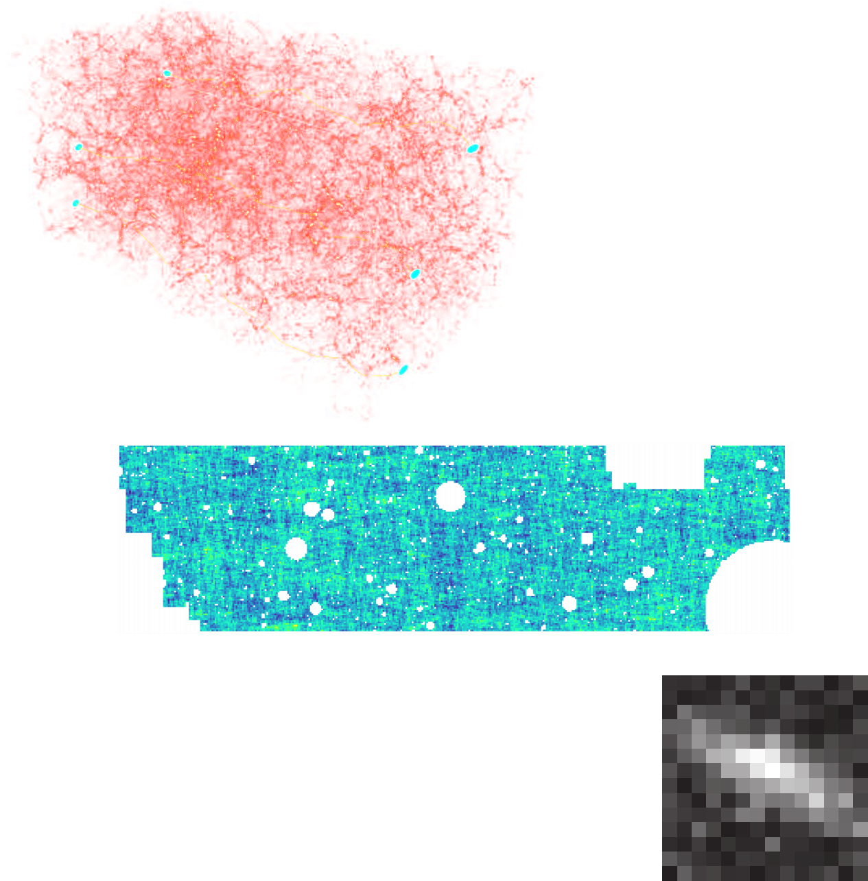
Gravitational Lensing as an Inverse Problem
Shear $\gamma$
![]()
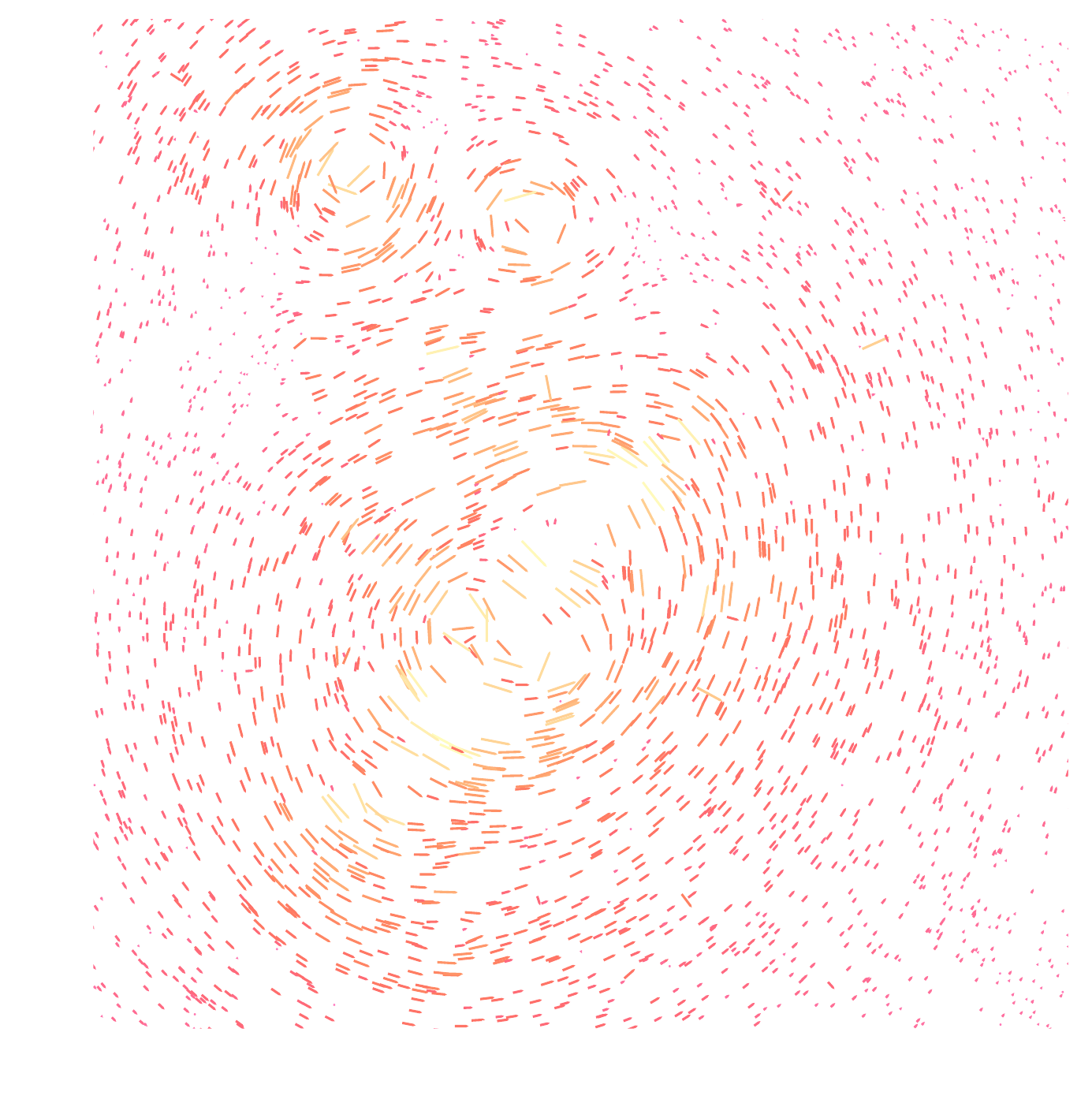
Convergence $\kappa$
![]()
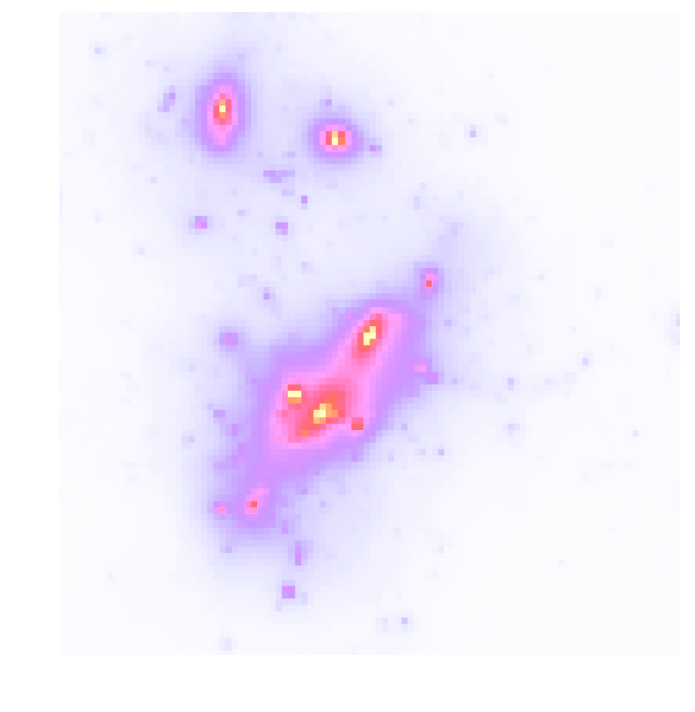
$$\gamma_1 = \frac{1}{2} (\partial_1^2 - \partial_2^2) \ \Psi \quad;\quad \gamma_2 = \partial_1 \partial_2 \ \Psi \quad;\quad \kappa = \frac{1}{2} (\partial_1^2 + \partial_2^2) \ \Psi$$
$$\boxed{\gamma = \mathbf{P} \kappa}$$
Writing down the convergence map log posterior
$$ \log p( \kappa | e) = \underbrace{\log p(e | \kappa)}_{\simeq -\frac{1}{2} \parallel e - P \kappa \parallel_\Sigma^2} + \log p(\kappa) +cst $$- The likelihood term is known analytically, given to us by the physics of gravitational lensing.
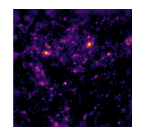
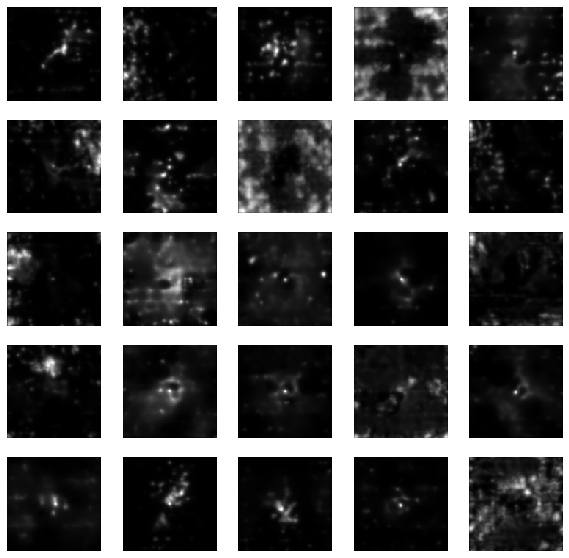
- There is no close form expression for the prior on dark matter maps $\kappa$.
However:- We do have access to samples of full implicit prior through simulations: $X = \{x_0, x_1, \ldots, x_n \}$ with $x_i \sim \mathbb{P}$
![]()
- We do have access to samples of full implicit prior through simulations: $X = \{x_0, x_1, \ldots, x_n \}$ with $x_i \sim \mathbb{P}$
$\Longrightarrow$ Our strategy: Learn the prior from simulation,
and then sample the full posterior.
How do you do this in practice in very high dimensional problems?
First realization: The score is all you need!
- Whether you are looking for the MAP or sampling with HMC or MALA, you
only need access to the score of the posterior:
$$\frac{\color{orange} d \color{orange}\log \color{orange}p\color{orange}(\color{orange}x \color{orange}|\color{orange} y\color{orange})}{\color{orange}
d
\color{orange}x}$$
- Gradient descent: $x_{t+1} = x_t + \tau \nabla_x \log p(x_t | y) $
- Langevin algorithm: $x_{t+1} = x_t + \tau \nabla_x \log p(x_t | y) + \sqrt{2\tau} n_t$
- The score of the full posterior is simply: $$\nabla_x \log p(x |y) = \underbrace{\nabla_x \log p(y |x)}_{\mbox{known explicitly}} \quad + \quad \underbrace{\nabla_x \log p(x)}_{\mbox{known implicitly}}$$ $\Longrightarrow$ "all" we have to do is model/learn the score of the prior.
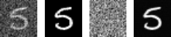
Neural Score Estimation by Denoising Score Matching (Vincent 2011)
- Denoising Score Matching: An optimal Gaussian denoiser learns the score of a given distribution.
- If $x \sim \mathbb{P}$ is corrupted by additional Gaussian noise $u \in \mathcal{N}(0, \sigma^2)$ to yield $$x^\prime = x + u$$
- Let's consider a denoiser $r_\theta$ trained under an $\ell_2$ loss: $$\mathcal{L}=\parallel x - r_\theta(x^\prime, \sigma) \parallel_2^2$$
- The optimal denoiser $r_{\theta^\star}$ verifies: $$\boxed{\boldsymbol{r}_{\theta^\star}(\boldsymbol{x}', \sigma) = \boldsymbol{x}' + \sigma^2 \nabla_{\boldsymbol{x}} \log p_{\sigma^2}(\boldsymbol{x}')}$$
$\boldsymbol{x}'$
$\boldsymbol{x}$
$\boldsymbol{x}'- \boldsymbol{r}^\star(\boldsymbol{x}', \sigma)$
$\boldsymbol{r}^\star(\boldsymbol{x}', \sigma)$
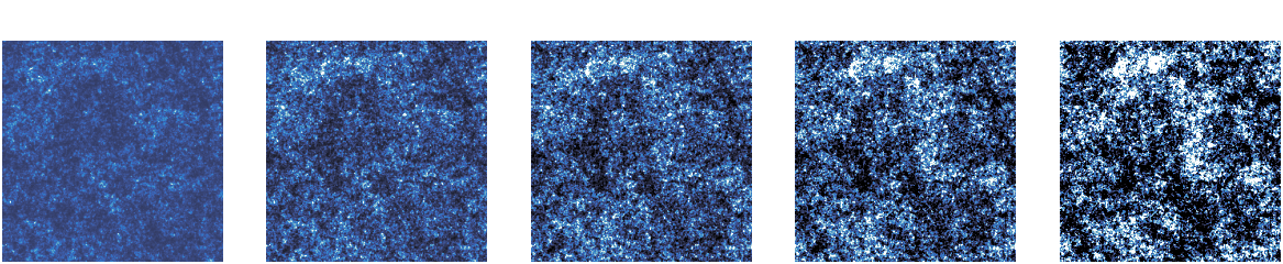
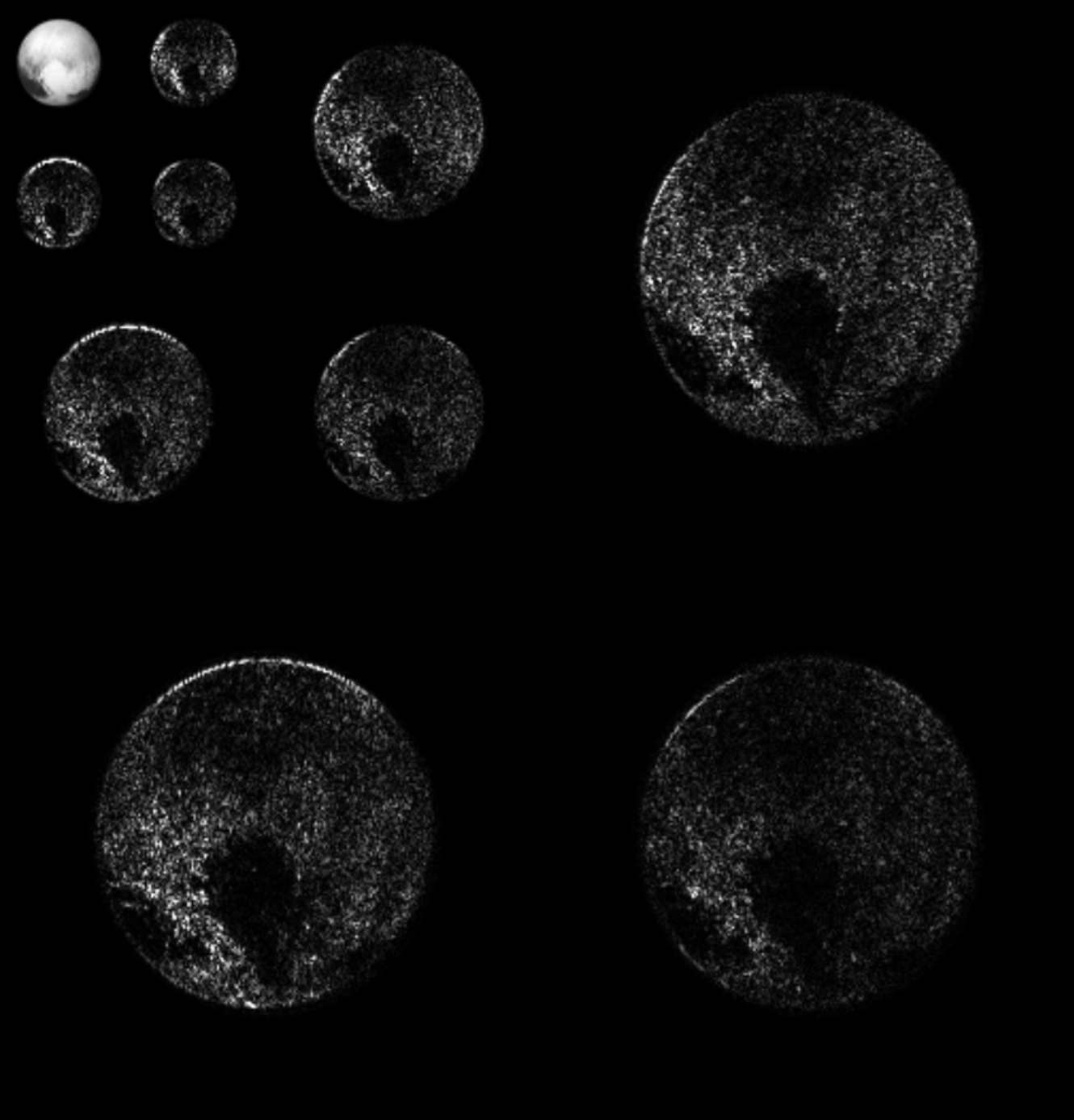
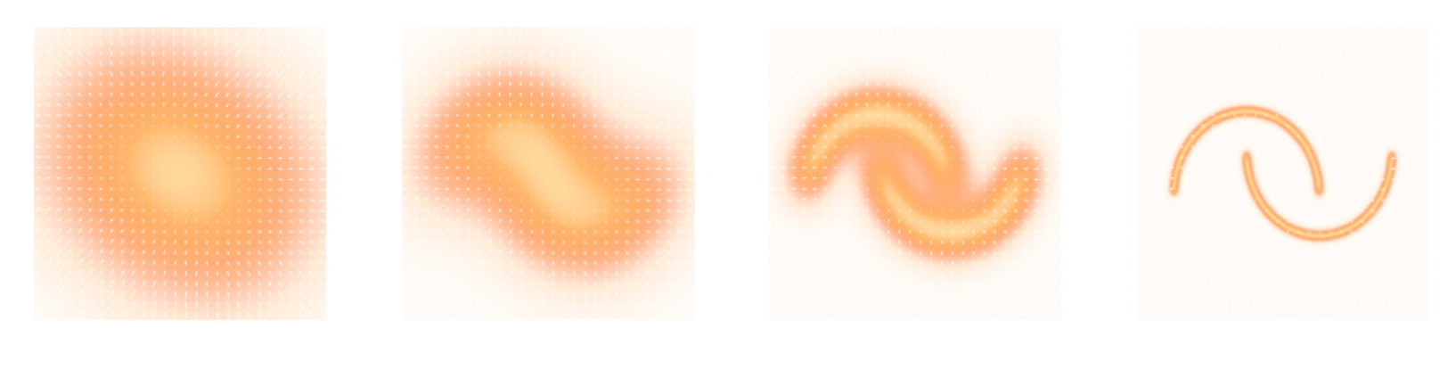
Second Realization: Annealing is everything!
- Even with knowledge of the score, sampling in high number of dimensions is difficult!
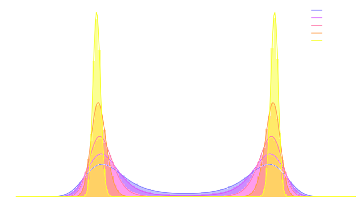
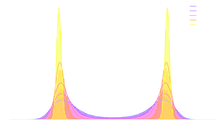
- Convolving a target distribution $p$ with a noise kernel, makes $p_\sigma(x) = \int \mathcal{N}(x; x^\prime, \sigma^2) (x^\prime) d x^{\prime}$ it much better behaved
$$\sigma_1 > \sigma_2 > \sigma_3 > \sigma_4 $$
![]()
- Hints to running many MCMC chains in parallel, progressively annealing the $\sigma$ to 0, keep last point in the chain as independent sample.
Score-Based Generative Modeling Song et al. (2021)
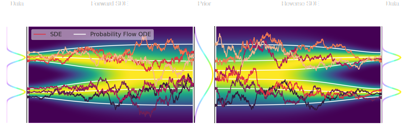
- The SDE defines a marginal distribution $p_t(x)$ as the convolution of the target distribution $p(x)$ with a noise kernel $p_{t|s}(\cdot | x_s)$: $$p_t(x) = \int p(x_s) p_{t|s}(x | x_s) d x_s$$
- For a given forward SDE that evolves $p(x)$ to $p_T(x)$, there exists a reverse SDE that evolves $p_T(x)$ back into $p(x)$. It involves having access to the marginal score $\nabla_x \log_t p(x)$.
Example of one chain during annealing
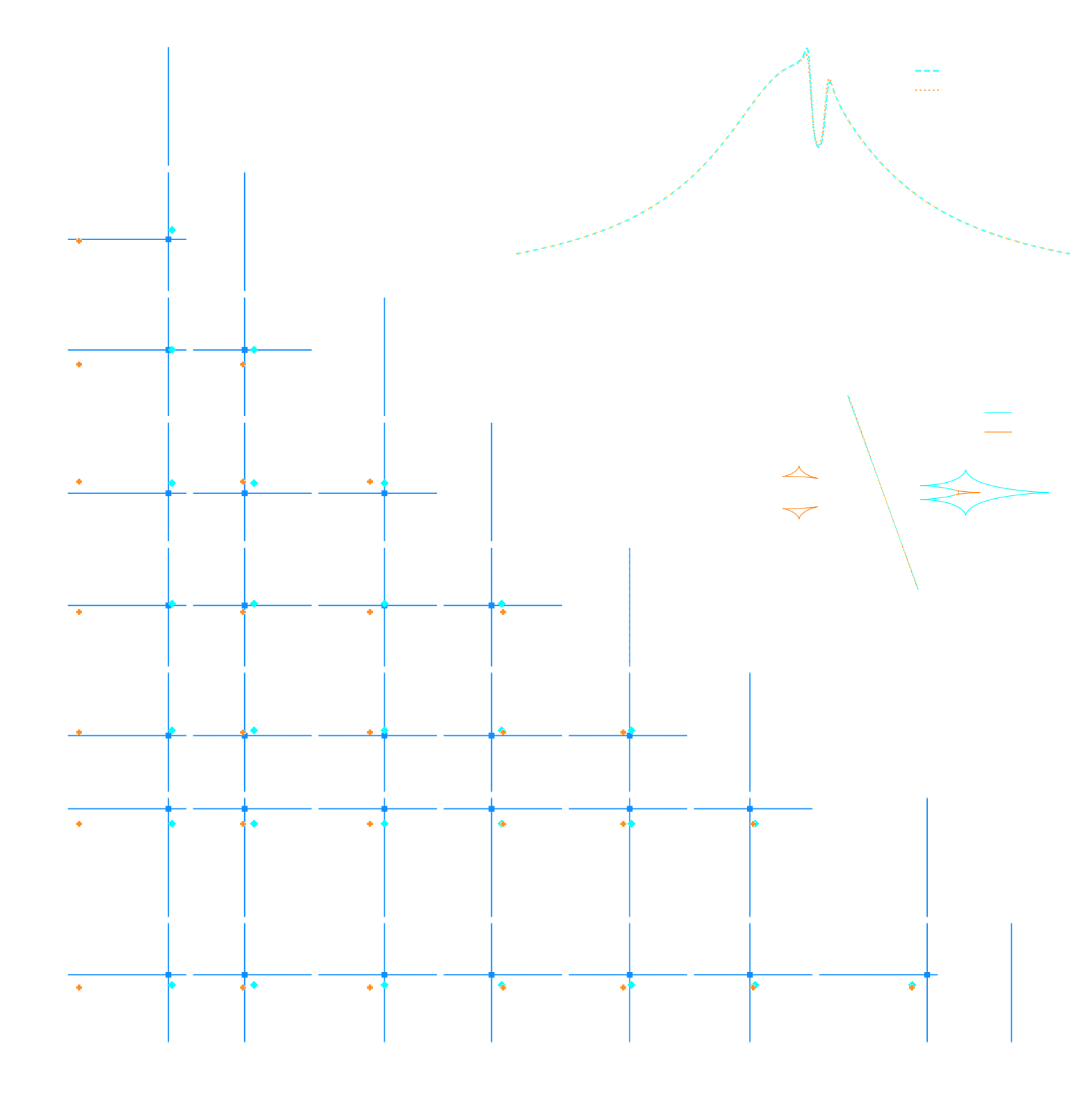
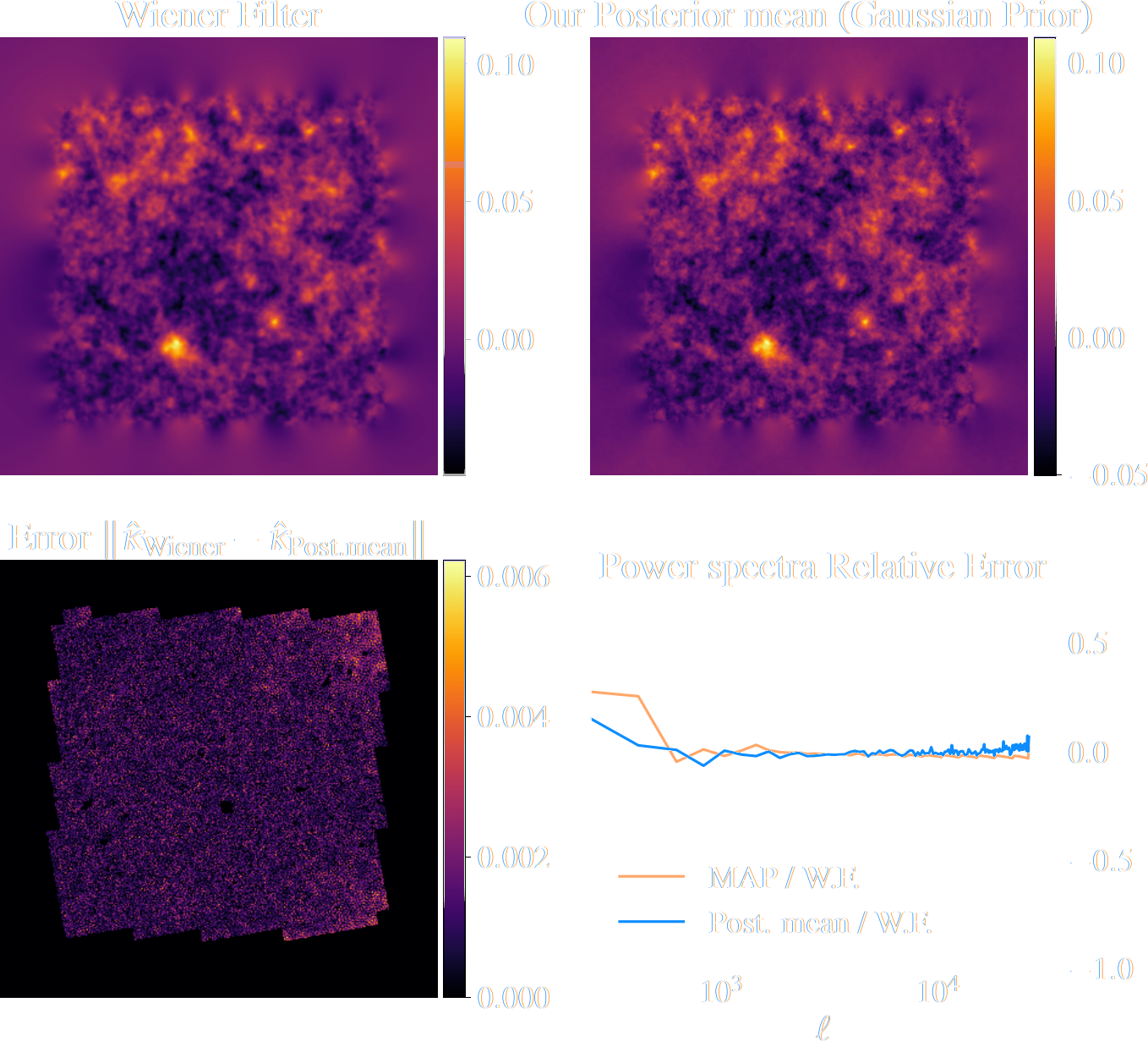
Validating Posterior Sampling under a Gaussian prior
Some details: We don't actually know the marginal posterior score!
- We know the following quantities:
- Annealed likelihood (analytically): $p_\sigma(y | x) = \mathcal{N}(y; \mathbf{A} x, \mathbf{\Sigma} + \sigma^2 \mathbf{I})$
- Annealed prior score (by score matching): $\nabla_x \log p_\sigma(x)$
- But, unfortunately: $\boxed{p_\sigma(x|y) \neq p_\sigma(y|x) \ p_\sigma(x)}$ $\Longrightarrow$ We don't know the marginal posterior score!
- We cannot use the reverse SDE/ODE of diffusion models to sample from the posterior. $$\mathrm{d} x = [f(x, t) - g^2(t) \underbrace{\nabla_x \log p_t(x|y)}_{\mbox{unknown}} ] \mathrm{d}t + g(t) \mathrm{d} w$$
Proposed sampling strategy
- Even if not equivalent to the marginal posterior score, $\nabla_x \log p_{\sigma^2}(y | x) + \nabla_x \log p_{\sigma^2}(x)$ still
has good properties:
- Tends to an isotropic Gaussian distribution for large $\sigma$
- Corresponds to the target posterior for $\sigma=0$
- If we simulate this SDE sufficiently slowly (i.e. timescale of change of $\sigma$ is much larger than the timescale of the SDE) we can expect to sample from the target posterior.
$\Longrightarrow$ In practice, we sample the annealed distribution using an Hamiltonian Monte-Carlo,
with discrete annealing steps.
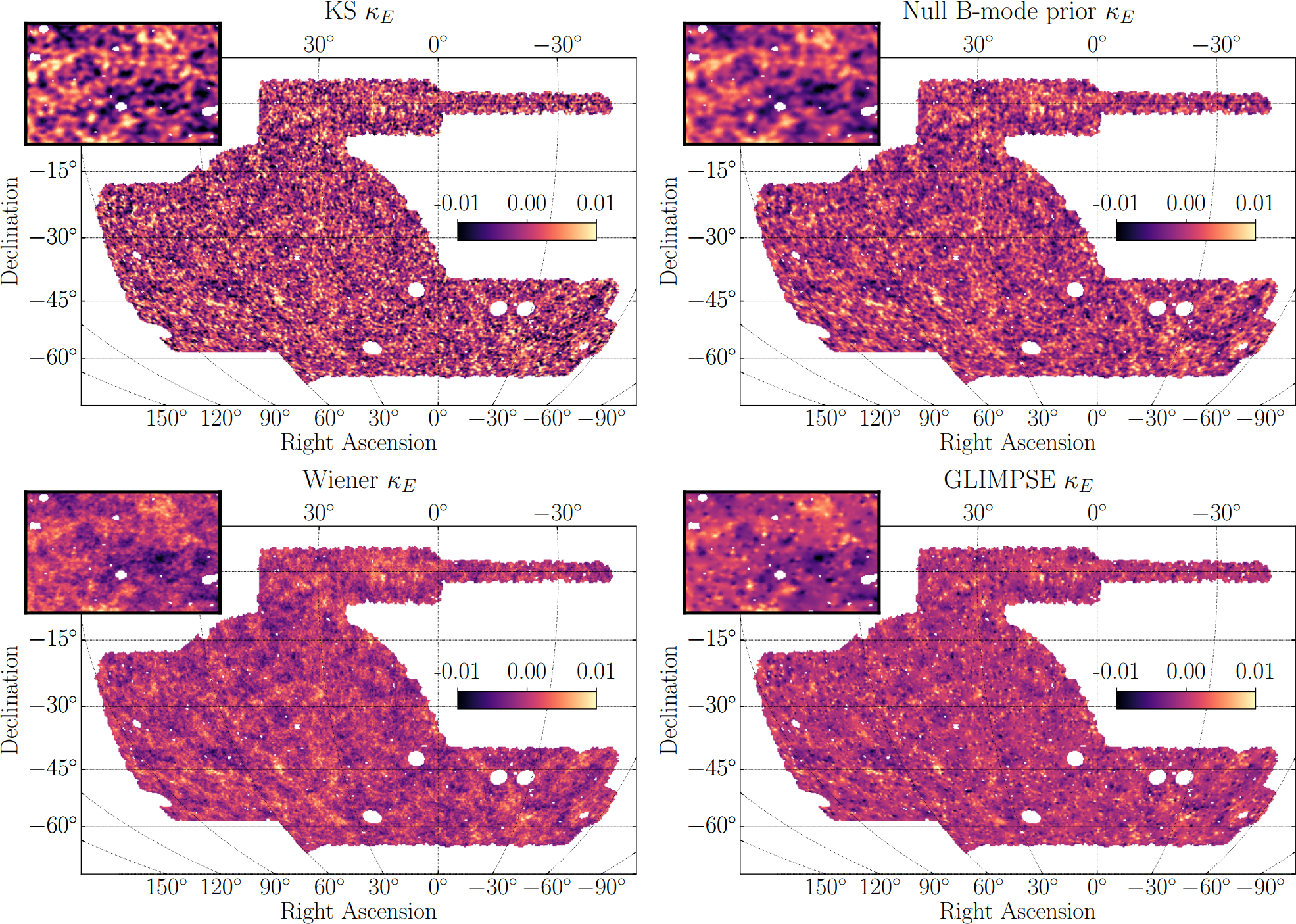
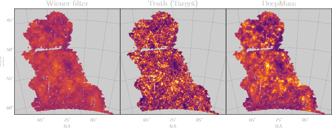
Illustration on $\kappa$-TNG simulations
Remy, Lanusse, et al. (2022) 
True convergence map
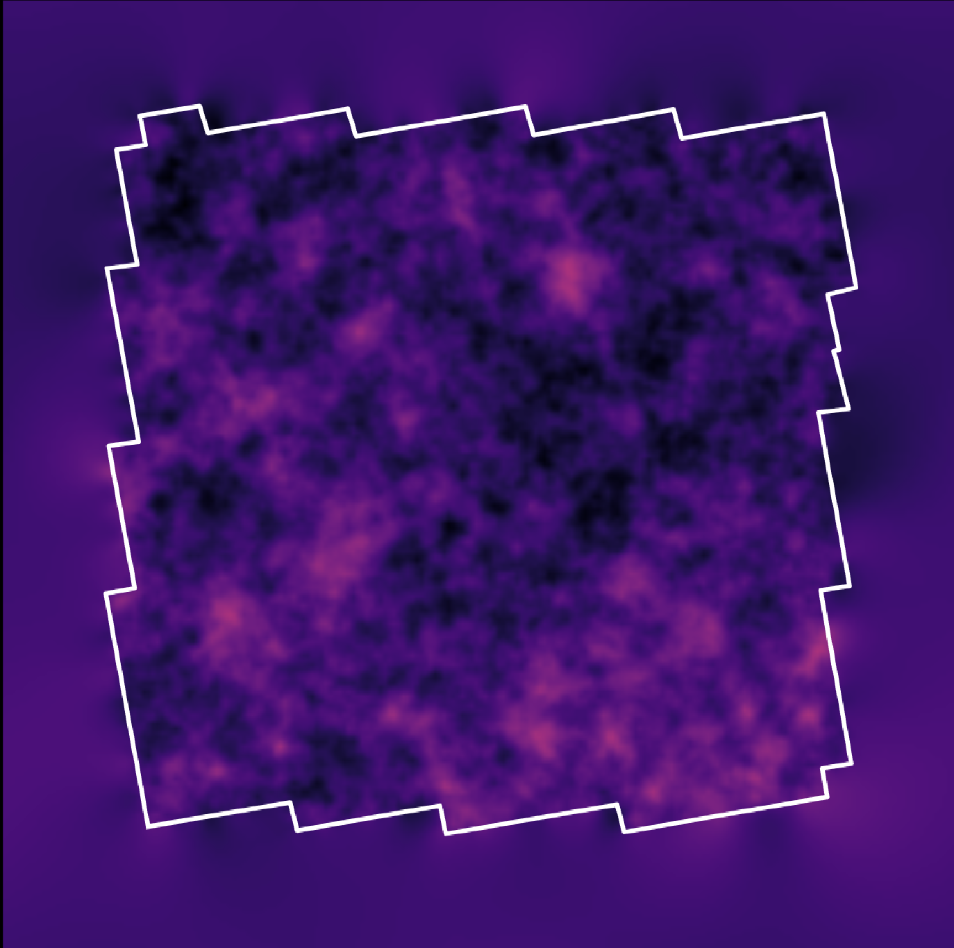
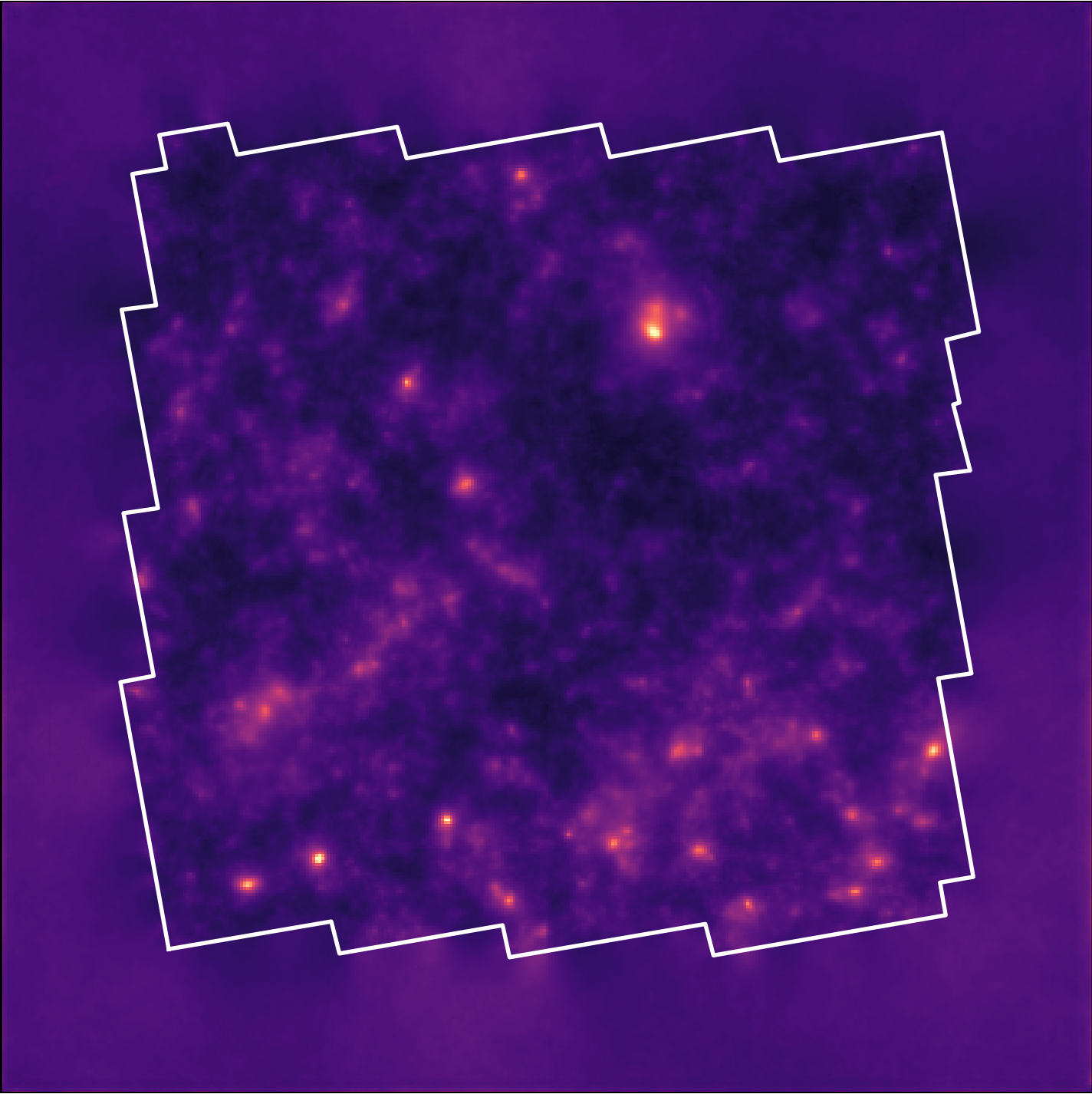
Traditional Kaiser-Squires
Wiener Filter
Posterior Mean (ours)
Posterior samples
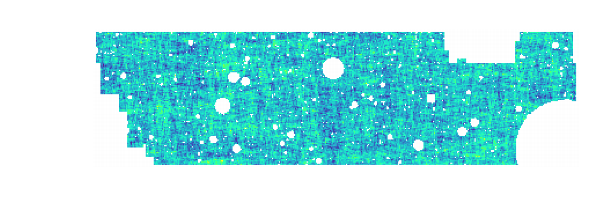
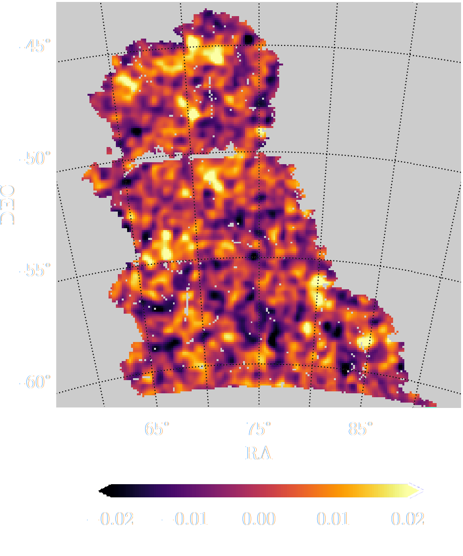
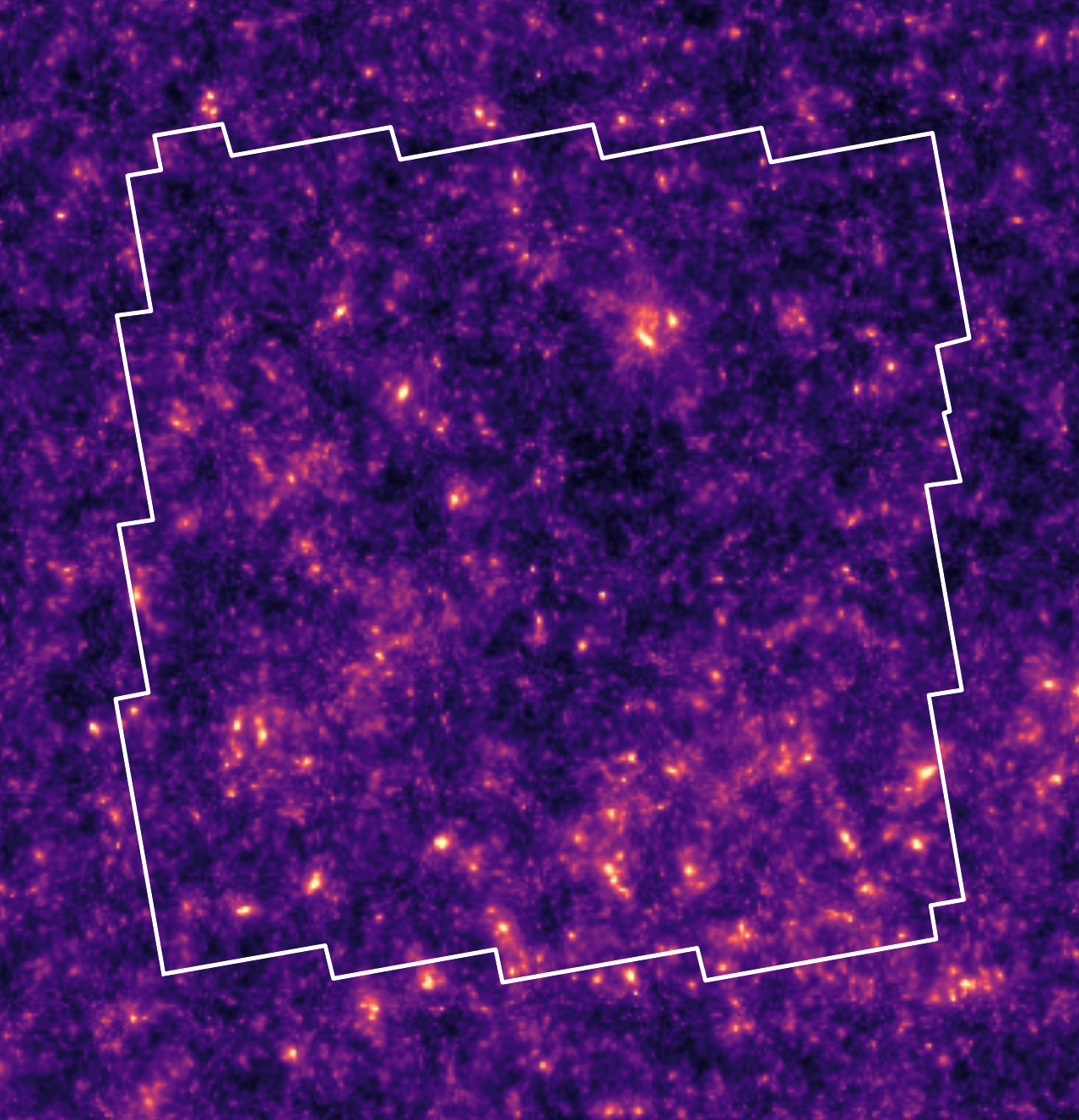
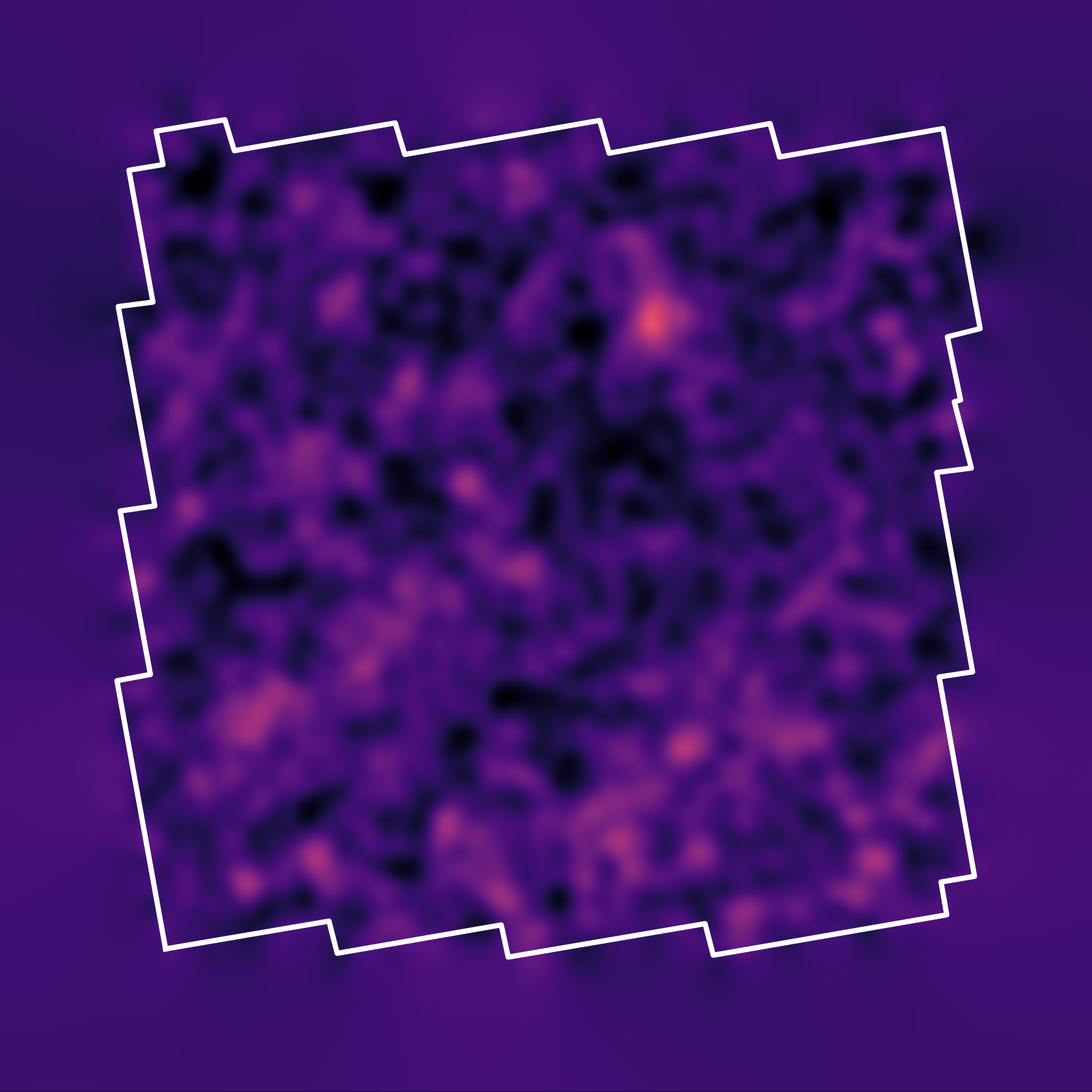
Reconstruction of the HST/ACS COSMOS field
- COSMOS shear data from Schrabback et al. 2010
- Prior learned from $\kappa$-TNG simulation from Osato et al. 2021.
Massey et al. (2007)
![]()
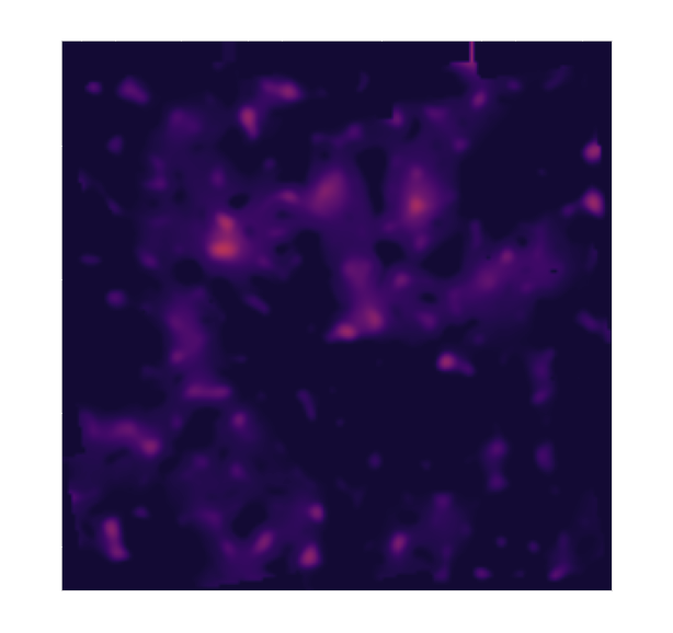
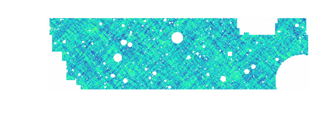
Remy et al. (2022) Posterior mean
![]()
Remy et al. (2022) Posterior samples
![]()
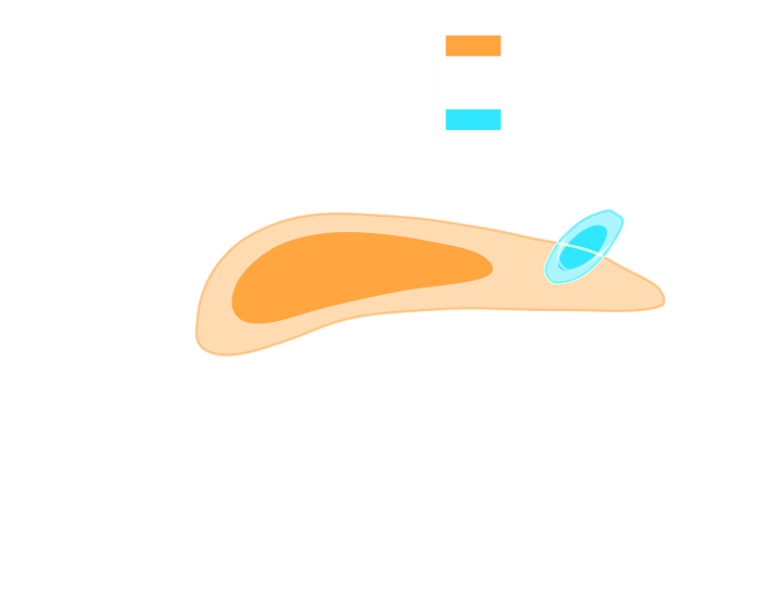
Inference over hybrid physical/deep learning models
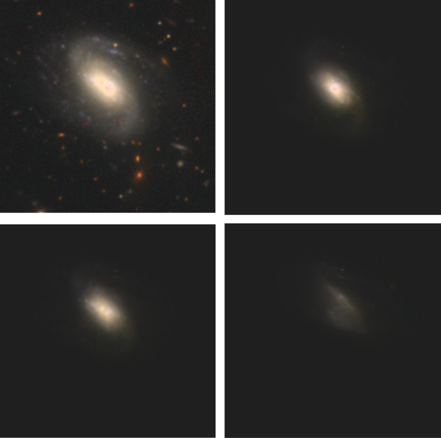
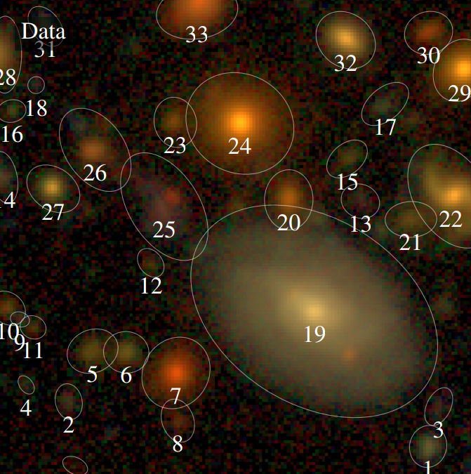
Impact of galaxy morphology on shape measurement
Mandelbaum, et al. (2013), Mandelbaum, et al. (2014)
$\Longrightarrow$ Let's learn a prior from this implicit distribution!
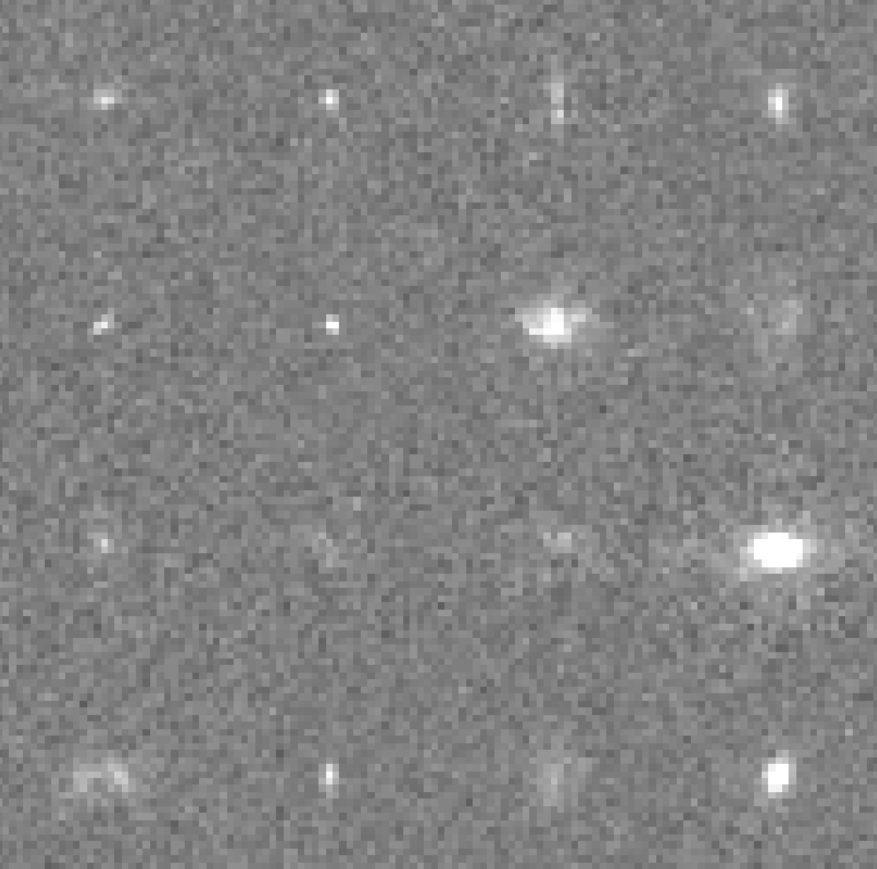
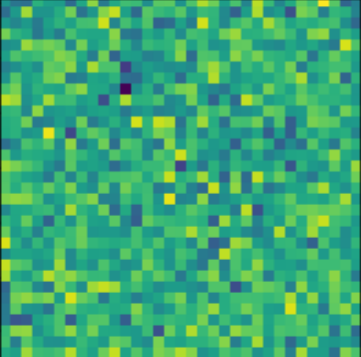
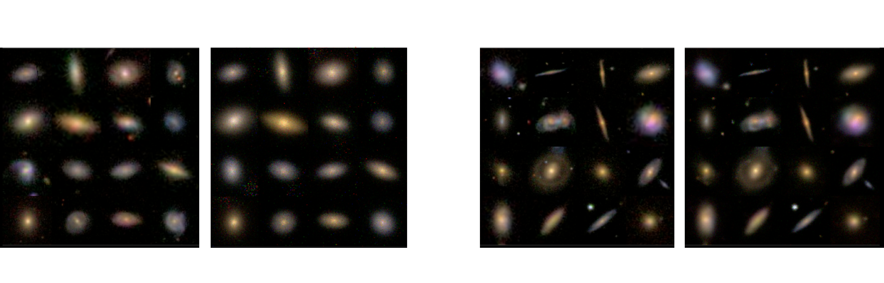
Complications specific to astronomical images: spot the differences!
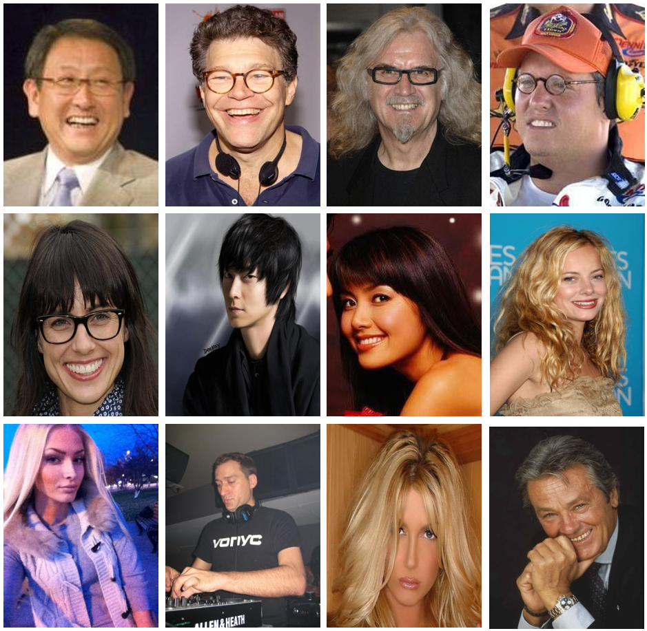
CelebA
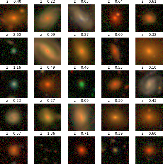
HSC PDR-2 wide
- There is noise
- We have a Point Spread Function (instrumental response)
A Physicist's approach: let's build a model

$\longrightarrow$
$g_\theta$
$g_\theta$
$\longrightarrow$
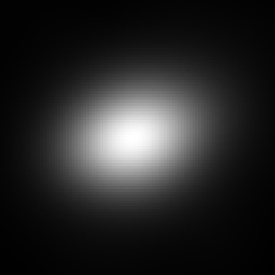
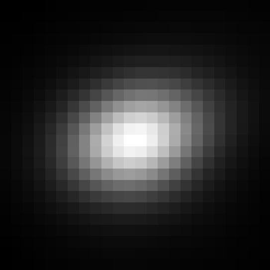
PSF
PSF
$\longrightarrow$
Pixelation
Pixelation
$\longrightarrow$
Noise
Noise
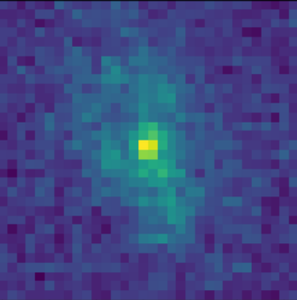
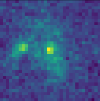
Probabilistic model
$$ x \sim ? $$
$$ x \sim \mathcal{N}(z, \Sigma) \quad z \sim ? $$
latent $z$ is a denoised galaxy image
latent $z$ is a denoised galaxy image
$$ x \sim \mathcal{N}( \mathbf{P} z, \Sigma) \quad z \sim ?$$
latent $z$ is a super-resolved and denoised galaxy image
latent $z$ is a super-resolved and denoised galaxy image
$$ x \sim \mathcal{N}( \mathbf{P} (\Pi \ast z), \Sigma) \quad z \sim ? $$
latent $z$ is a deconvolved, super-resolved, and denoised galaxy image
latent $z$ is a deconvolved, super-resolved, and denoised galaxy image
$$ x \sim \mathcal{N}( \mathbf{P} (\Pi \ast g_\theta(z)), \Sigma) \quad z \sim \mathcal{N}(0, \mathbf{I}) $$
latent $z$ is a Gaussian sample
$\theta$ are parameters of the model
latent $z$ is a Gaussian sample
$\theta$ are parameters of the model
$\Longrightarrow$ Decouples the morphology model from the observing conditions.
How to train your dragon model
- Training the generative amounts to finding $\theta_\star$ that
maximizes the marginal likelihood of the model:
$$p_\theta(x | \Sigma, \Pi) = \int \mathcal{N}( \Pi \ast g_\theta(z), \Sigma) \ p(z) \ dz$$
$\Longrightarrow$ This is generally intractable
- Efficient training of parameter $\theta$ is made possible by Amortized Variational Inference.
Auto-Encoding Variational Bayes (Kingma & Welling, 2014)
- We introduce a parametric distribution $q_\phi(z | x, \Pi, \Sigma)$ which aims to model the posterior $p_{\theta}(z | x, \Pi, \Sigma)$.
- Working out the KL divergence between these two distributions leads to: $$\log p_\theta(x | \Sigma, \Pi) \quad \geq \quad - \mathbb{D}_{KL}\left( q_\phi(z | x, \Sigma, \Pi) \parallel p(z) \right) \quad + \quad \mathbb{E}_{z \sim q_{\phi}(. | x, \Sigma, \Pi)} \left[ \log p_\theta(x | z, \Sigma, \Pi) \right]$$ $\Longrightarrow$ This is the Evidence Lower-Bound, which is differentiable with respect to $\theta$ and $\phi$.
The famous Variational Auto-Encoder
$$\log p_\theta(x| \Sigma, \Pi ) \geq - \underbrace{\mathbb{D}_{KL}\left( q_\phi(z | x, \Sigma, \Pi) \parallel p(z) \right)}_{\mbox{code regularization}} + \underbrace{\mathbb{E}_{z \sim q_{\phi}(. | x, \Sigma, \Pi)} \left[ \log p_\theta(x | z, \Sigma, \Pi) \right]}_{\mbox{reconstruction error}} $$
Sampling from the model
 Woups... what's going on?
Tradeoff between code regularization and image quality
$$\log p_\theta(x| \Sigma, \Pi ) \geq - \underbrace{\mathbb{D}_{KL}\left( q_\phi(z | x, \Sigma, \Pi) \parallel p(z) \right)}_{\mbox{code regularization}} + \underbrace{\mathbb{E}_{z \sim q_{\phi}(. | x, \Sigma, \Pi)} \left[ \log p_\theta(x | z, \Sigma, \Pi) \right]}_{\mbox{reconstruction error}} $$
Latent space modeling with Normalizing Flows
$\Longrightarrow$ All we need to do is sample from the aggregate posterior of the data instead of sampling from the prior.
Dinh et al. 2016
Normalizing Flows
- Assumes a bijective mapping between data space $x$ and latent space $z$ with prior $p(z)$: $$ z = f_{\theta} ( x ) \qquad \mbox{and} \qquad x = f^{-1}_{\theta}(z)$$
- Admits an explicit marginal likelihood: $$ \log p_\theta(x) = \log p(z) + \log \left| \frac{\partial f_\theta}{\partial x} \right|(x) $$
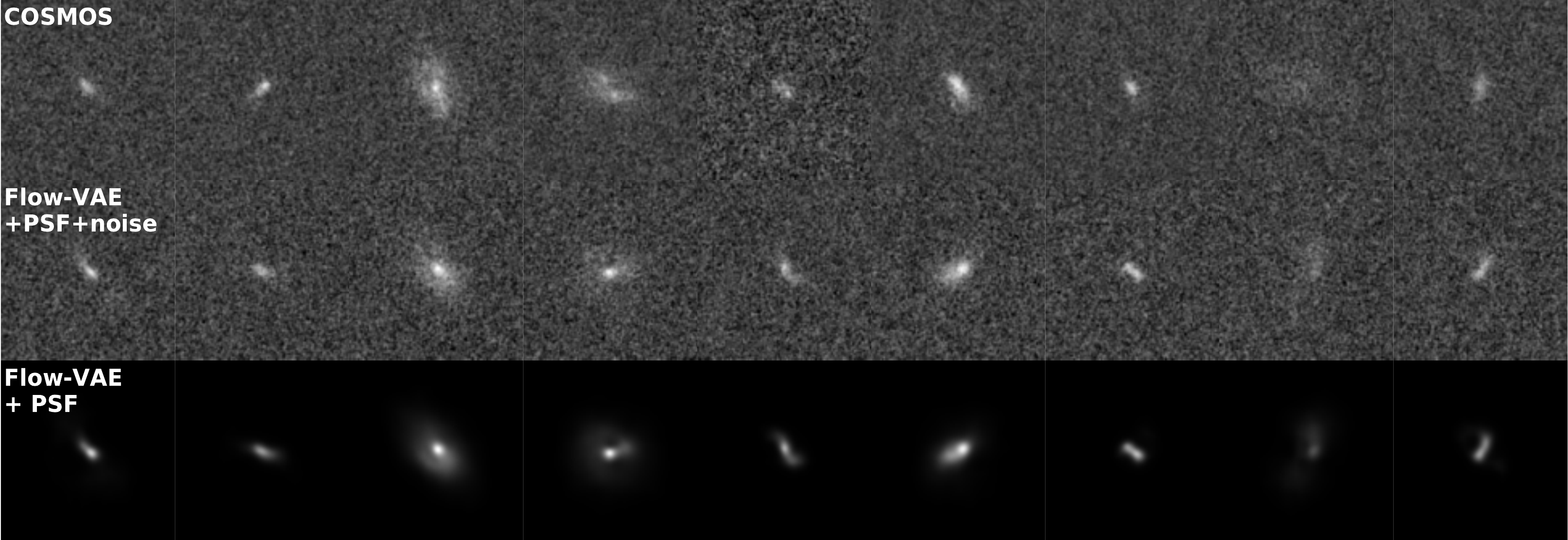
Flow-VAE samples
How do I use my generative model to infer gravitational lensing?
Let's again think as physicists
$\longrightarrow$
$g_\theta$
$g_\theta$
$\longrightarrow$
shear $\gamma$
shear $\gamma$
$\longrightarrow$
PSF
PSF
$\longrightarrow$
Noise
Noise
Probabilistic model
$$ x \sim \mathcal{N}(\Pi \ast
(g_\theta(z) \otimes \gamma), \Sigma) \quad z \sim \mathcal{N}(0,
\mathbf{I}) $$
latent $z$ are morphological parameters
$\theta$ are global parameters of the model
$\gamma$ are shear parameters
latent $z$ are morphological parameters
$\theta$ are global parameters of the model
$\gamma$ are shear parameters
$\Longrightarrow$ We have a hybrid probabilistic model, with the known physics of lensing and of the instrument, and
learned morphology model.
Joint inference using a parametric model for the morphology
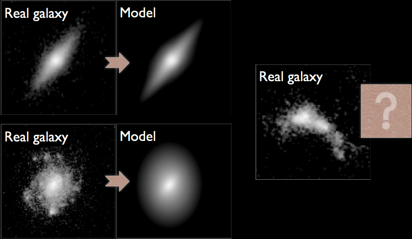
Let's assume that $g(z)$ is a sersic model, i.e. $z = \{n, r_\text{hlr}, F, e_1, e_2, s_x, s_y\}$ and
$$g(z) = F \times I_0 \exp \left( -b_n \left[\left( \frac{r}{r_\text{hlr}}\right)^{\frac{1}{n}} -1\right] \right)$$
We need a more realistic model of galaxy morphology
The joint inference of $p(z, \gamma | \mathcal{D})$ leads to a biased posterior...
Marginal shear posterior $p(\gamma|\mathcal{D})$
Maximum a posteriori fit and residuals
Marginal shear posterior $p(\gamma|\mathcal{D})$
Maximum a posteriori fit and residuals
We need a more realistic model of galaxy morphology
Joint inference using a generative model for the morpholgy
Remy, Lanusse, Starck (2022)

Let's use a learned $g_\theta(z)$
The joint inference of $p(z, \gamma | \mathcal{D})$ leads to an unbiased posterior!
Marginal shear posterior $p(\gamma|\mathcal{D})$
Maximum a posteriori fit and residuals
Marginal shear posterior $p(\gamma|\mathcal{D})$
Maximum a posteriori fit and residuals
Takeaway message
- We have introduce an hybrid physical/deep learning model
- Incorporate prior astrophysical knowledge as a data-driven prior, from degraded observations.
$\Longrightarrow$ Learned a deconvolved distribution. - Interpretable in terms of physical quantities of the astronomical scene
- This is a specific illustration, but the same idea can apply to many other physical models that are not fully well specified.
- Incorporate prior astrophysical knowledge as a data-driven prior, from degraded observations.