Taming Implicit Distributions with Generative Modeling
SLAC Summer Institute, August 2023
François Lanusse


slides at eiffl.github.io/talks/SSI2023
the Rubin Observatory Legacy Survey of Space and Time
- 1000 images each night, 15 TB/night for 10 years
- 18,000 square degrees, observed once every few days
- Tens of billions of objects, each one observed $\sim1000$ times
Previous generation survey: SDSS
Image credit: Peter Melchior
Current generation survey: DES
Image credit: Peter Melchior
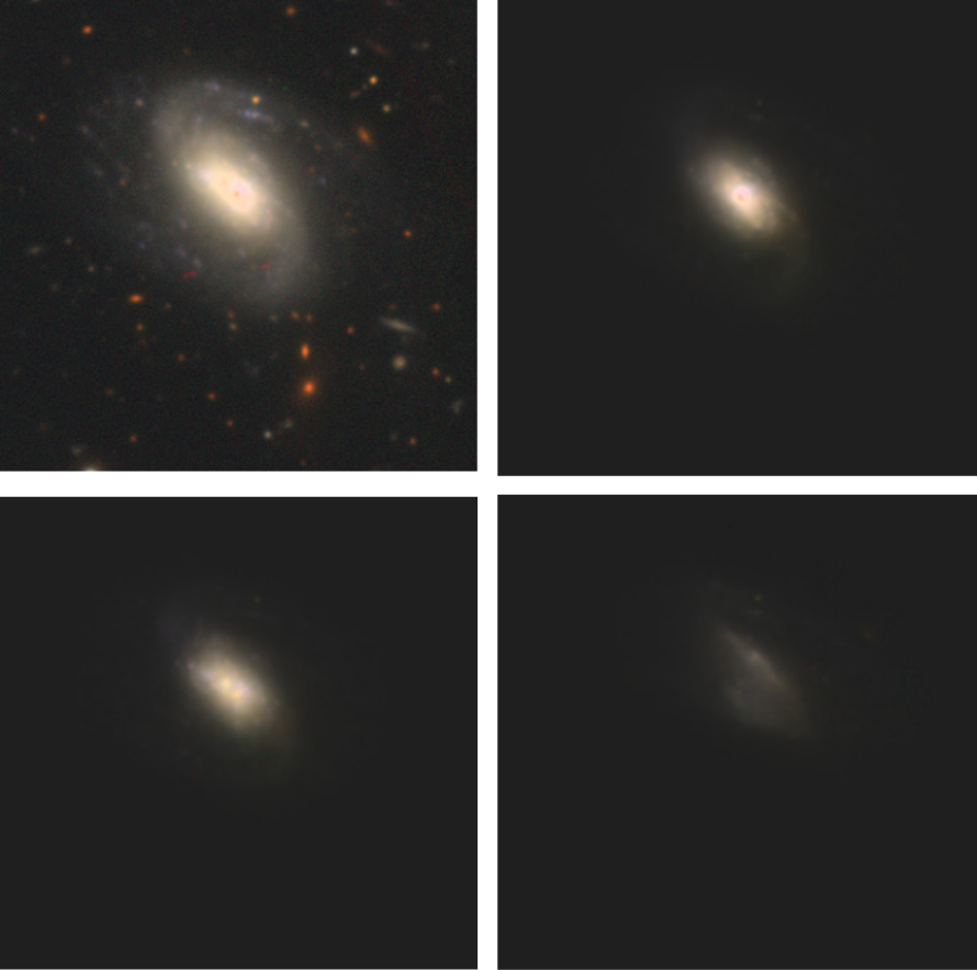
LSST precursor survey: HSC
Image credit: Peter Melchior
We need to rethink all stages of data analysis
Bosch et al. 2017
Jeffrey, Lanusse, et al. 2020
Cheng et al. 2020
- Galaxies are no longer blobs.
- Signals are no longer Gaussian.
- Cosmological likelihoods are no longer tractable.
$\Longrightarrow$ This is the end of the analytic era...
... but the beginning of the data-driven era
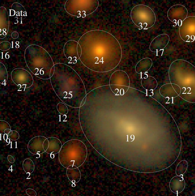
Case I: Examples from data, no accurate physical model
![]()
Mandelbaum et al. 2014
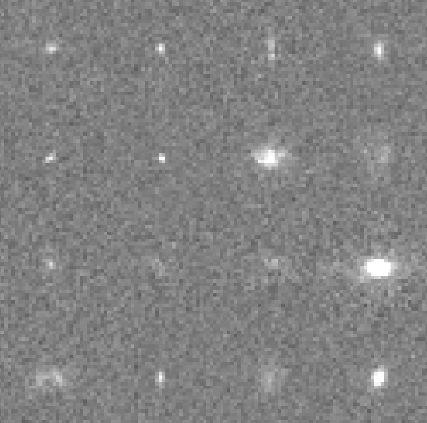
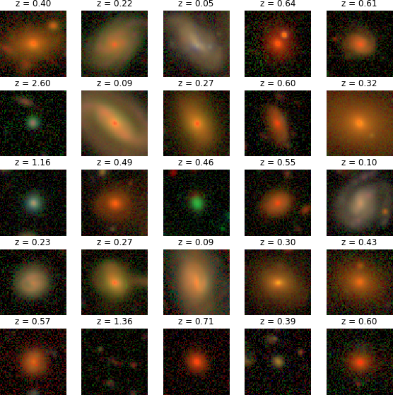
Case II: Physical model only available as a simulator
![]()
Osato et al. 2020
$\Longrightarrow$ Examples of implicit distributions: we have access to samples $\{x_0, x_1, \ldots, x_n \}$
but we cannot evaluate $p(x)$.
How can we leverage implicit distributions
for physical Bayesian inference?
The answer is: Deep Generative Modeling
- The goal of generative modeling is to learn an implicit distribution $\mathbb{P}$ from which the training set $X = \{x_0, x_1, \ldots, x_n \}$ is drawn.
- Usually, this means building a parametric model $\mathbb{P}_\theta$ that tries to be close to $\mathbb{P}$.

True $\mathbb{P}$

Samples $x_i \sim \mathbb{P}$

Model $\mathbb{P}_\theta$
- Once trained, you can typically sample from $\mathbb{P}_\theta$ and/or evaluate the likelihood $p_\theta(x)$.
In the rest of this talk
Main idea: Use generative models to complement physical models with implicit distributions, and perform inference in a Bayesian context.
Several examples today:
- Implicit Distributions as Priors in
Inverse Problems - Hybrid Physical/Data-Driven Hierarchical
Bayesian Models
Implicit Distributions as Priors in
Inverse Problems
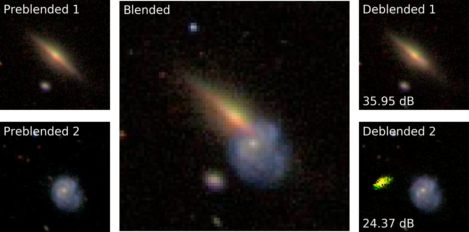
Branched GAN model for deblending (Reiman & Göhre, 2018)
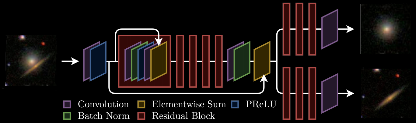
The issue with using deep learning as a black-box
- No explicit control of noise, PSF, number of sources.
- Model would have to be retrained for all observing configurations
- No guarantees on the network output (e.g. flux preservation, artifacts)
- No proper uncertainty quantification.
Linear inverse problems
$\boxed{y = \mathbf{A}x + n}$$\mathbf{A}$ is known and encodes our physical understanding of the problem.
$\Longrightarrow$ When non-invertible or ill-conditioned, the inverse problem is ill-posed with no unique solution $x$
 Deconvolution
 Inpainting
 Denoising
What Would a Bayesian Do?
$\boxed{y = \mathbf{A}x + n}$
$$ p(x | y) \propto p(y | x) \ p(x) $$
- $p(y | x)$ is the data likelihood, which contains the
physics
- $p(x)$ is our prior knowledge on the solution.
With these concepts in hand, we want to estimate the Maximum A Posteriori solution:
$$\hat{x} = \arg\max\limits_x \ \log p(y \ | \ x) + \log p(x)$$
For instance, if $n$ is Gaussian, $\hat{x} = \arg\max\limits_x \ - \frac{1}{2} \parallel y - \mathbf{A} x \parallel_{\mathbf{\Sigma}}^2 + \log p(x)$
$$\hat{x} = \arg\max\limits_x \ \log p(y \ | \ x) + \log p(x)$$
For instance, if $n$ is Gaussian, $\hat{x} = \arg\max\limits_x \ - \frac{1}{2} \parallel y - \mathbf{A} x \parallel_{\mathbf{\Sigma}}^2 + \log p(x)$
How do you choose the prior ?
Classical examples of signal priors
Sparse
![]()
$$ \log p(x) = \parallel \mathbf{W} x \parallel_1 $$
$$ \log p(x) = \parallel \mathbf{W} x \parallel_1 $$
Gaussian
![]() $$ \log p(x) = x^t \mathbf{\Sigma^{-1}} x $$
$$ \log p(x) = x^t \mathbf{\Sigma^{-1}} x $$
 $$ \log p(x) = x^t \mathbf{\Sigma^{-1}} x $$
Total Variation
![]() $$ \log p(x) = \parallel \nabla x \parallel_1 $$
$$ \log p(x) = \parallel \nabla x \parallel_1 $$
But what about this?
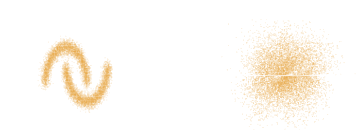
Getting started with Deep Priors: deep denoising example
$$ \boxed{{\color{Orchid} y} = {\color{SkyBlue} x} + n} $$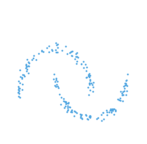
- Let us assume we have access to examples of $ {\color{SkyBlue} x}$ without noise.
- We learn the distribution of noiseless data $\log p_\theta(x)$ from samples using a deep generative model.
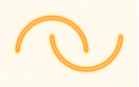
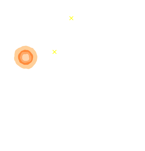
- The solution should lie on the realistic data
manifold, symbolized by the two-moons distribution.
We want to solve for the Maximum A Posterior solution:
$$\arg \max - \frac{1}{2} \parallel {\color{Orchid} y} - {\color{SkyBlue} x} \parallel_2^2 + \log p_\theta({\color{SkyBlue} x})$$ This can be done by gradient descent as long as one has access to the score function $\frac{\color{orange} d \color{orange}\log \color{orange}p\color{orange}(\color{orange}x\color{orange})}{\color{orange} d \color{orange}x}$.
Data-driven priors for astronomical inverse problems
Work in collaboration with
Peter Melchior, Fred Moolekamp, Remy Joseph
The Scarlet algorithm: deblending as an optimization problem
Melchior et al. 2018
$$ \mathcal{L} = \frac{1}{2} \parallel \mathbf{\Sigma}^{-1/2} (\ Y - P \ast A S \ ) \parallel_2^2 - \sum_{i=1}^K \log p_{\theta}(S_i) + \sum_{i=1}^K g_i(A_i) + \sum_{i=1}^K f_i(S_i)$$
Where for a $K$ component blend:
- $P$ is the convolution with the instrumental response
- $A_i$ are channel-wise galaxy SEDs, $S_i$ are the morphology models
- $\mathbf{\Sigma}$ is the noise covariance
- $\log p_\theta$ is a PixelCNN prior
- $f_i$ and $g_i$ are arbitrary additional non-smooth consraints, e.g. positivity, monotonicity...
PixelCNN: Likelihood-based Autoregressive generative model
Models the probability $p(x)$ of an image $x$ as:
$$ p_{\theta}(x) = \prod_{i=0}^{n} p_{\theta}(x_i | x_{i-1} \ldots x_0) $$
- $p_\theta(x)$ is explicit! We get a number out.
- We can train the model to learn a distribution of isolated galaxy images.
- We can then evaluate its gradient $\frac{\color{orange} d \color{orange}\log \color{orange}p\color{orange}(\color{orange}x\color{orange})}{\color{orange} d \color{orange}x}$.
van den Oord et al. 2016
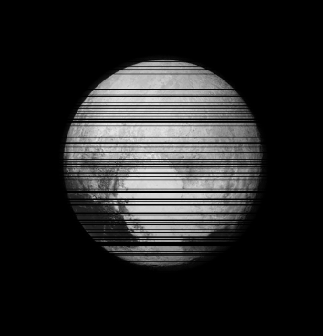
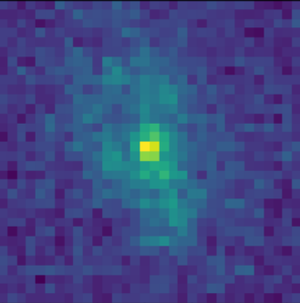
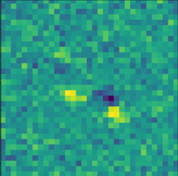
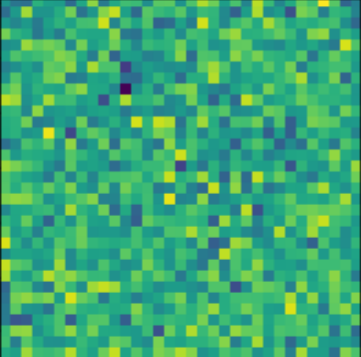
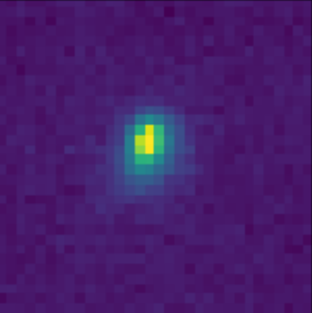
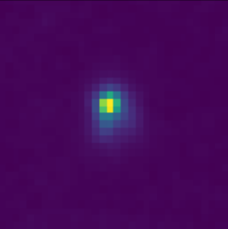
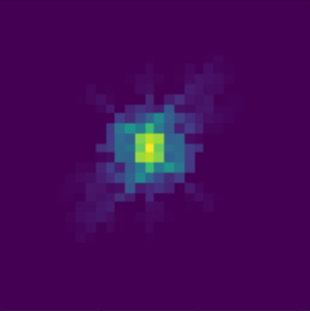
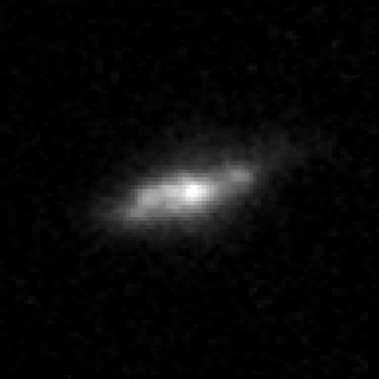
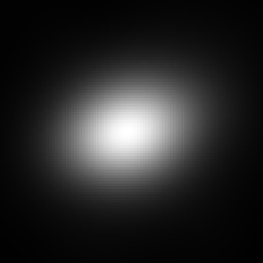
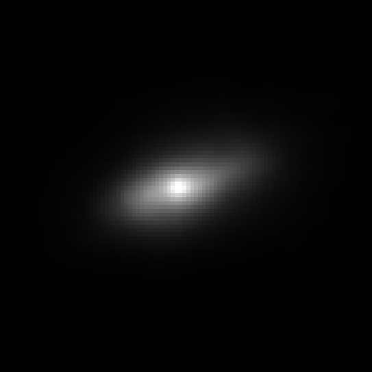
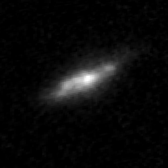
Training the morphology prior
Postage stamps of isolated COSMOS galaxies used for training, at Roman resolution and fixed fiducial PSF
isolated galaxy
![]() $\log p_\theta(x) = 3293.7$
$\log p_\theta(x) = 3293.7$
 $\log p_\theta(x) = 3293.7$
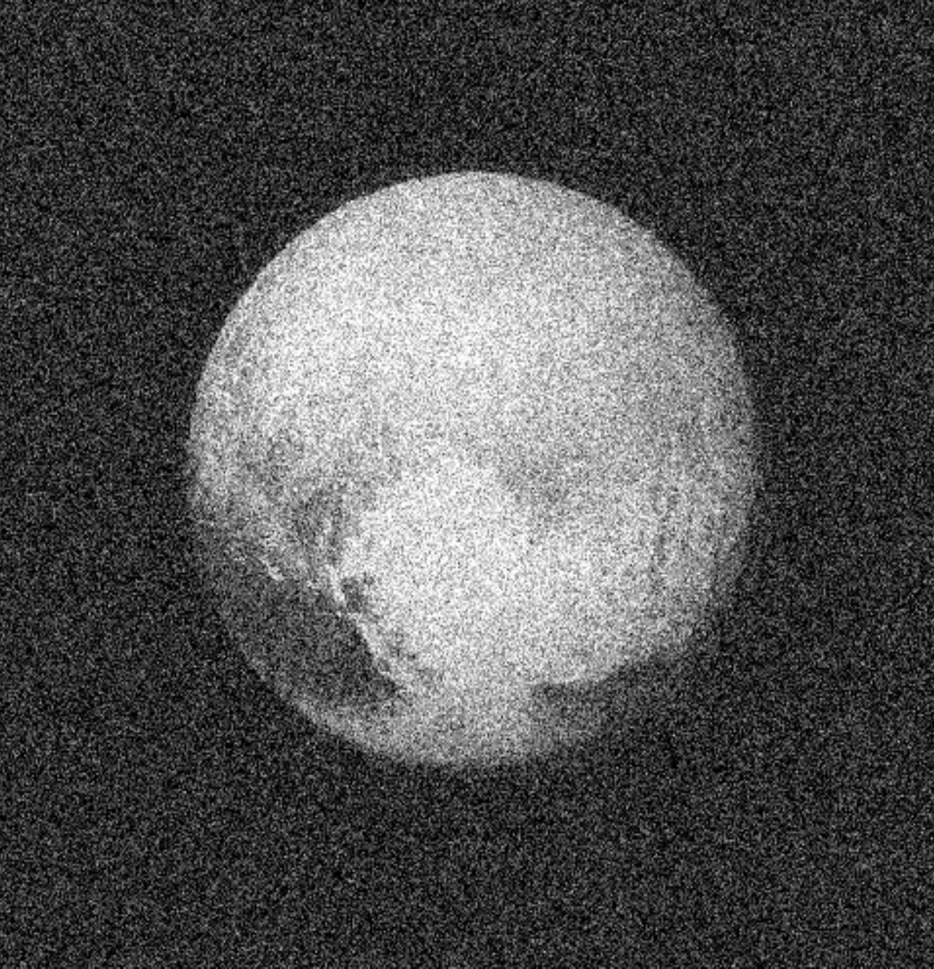
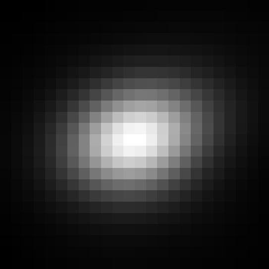
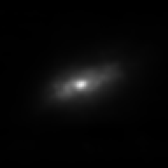
artificial blend
![]() $\log p_\theta(x) = 3100.5 $
$\log p_\theta(x) = 3100.5 $
 $\log p_\theta(x) = 3100.5 $
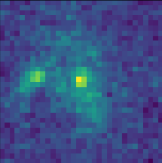
Scarlet in action
Input blend
![]()
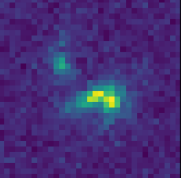
Solution
![]()
![]()
Residuals
![]()
![]()
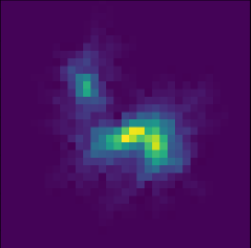
- Classic priors (monotonicity, symmetry).
- Deep Morphology prior.
True Galaxy
![]()
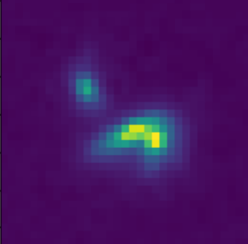
Deep Morphology Prior Solution
![]()
Monotonicity + Symmetry Solution
![]()
But what about uncertainties?
What Would a Bayesian Do?
$\boxed{y = \mathbf{A}x + n}$
$$ p(x | y) \propto p(y | x) \ p(x) $$
- $p(y | x)$ is the data likelihood, which contains the
physics
- $p(x)$ is our prior knowledge on the solution.
With these concepts in hand, we can:
- Estimate the Maximum A Posteriori solution: $$\hat{x} = \arg\max\limits_x \ \log p(y \ | \ x) + \log p(x)$$
- Estimate the full posterior p(x|y) with Markov Chain Monte-Carlo or Variational Inference methods
$\Longrightarrow$ Until very recently sampling from such posteriors in high number of dimensions remained very difficult!
First realization: The score is all you need!
- Whether you are looking for the MAP or sampling with HMC or MALA, you
only need access to the score of the posterior:
$$\frac{\color{orange} d \color{orange}\log \color{orange}p\color{orange}(\color{orange}x \color{orange}|\color{orange} y\color{orange})}{\color{orange}
d
\color{orange}x}$$
- Gradient descent: $x_{t+1} = x_t + \tau \nabla_x \log p(x_t | y) $
- Langevin algorithm: $x_{t+1} = x_t + \tau \nabla_x \log p(x_t | y) + \sqrt{2\tau} n_t$
- The score of the full posterior is simply: $$\nabla_x \log p(x |y) = \underbrace{\nabla_x \log p(y |x)}_{\mbox{known explicitly}} \quad + \quad \underbrace{\nabla_x \log p(x)}_{\mbox{known implicitly}}$$ $\Longrightarrow$ "all" we have to do is model/learn the score of the prior.
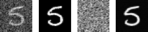
Neural Score Estimation by Denoising Score Matching (Vincent 2011)
- Denoising Score Matching: An optimal Gaussian denoiser learns the score of a given distribution.
- If $x \sim \mathbb{P}$ is corrupted by additional Gaussian noise $u \in \mathcal{N}(0, \sigma^2)$ to yield $$x^\prime = x + u$$
- Let's consider a denoiser $r_\theta$ trained under an $\ell_2$ loss: $$\mathcal{L}=\parallel x - r_\theta(x^\prime, \sigma) \parallel_2^2$$
- The optimal denoiser $r_{\theta^\star}$ verifies: $$\boxed{\boldsymbol{r}_{\theta^\star}(\boldsymbol{x}', \sigma) = \boldsymbol{x}' + \sigma^2 \nabla_{\boldsymbol{x}} \log p_{\sigma^2}(\boldsymbol{x}')}$$
$\boldsymbol{x}'$
$\boldsymbol{x}$
$\boldsymbol{x}'- \boldsymbol{r}^\star(\boldsymbol{x}', \sigma)$
$\boldsymbol{r}^\star(\boldsymbol{x}', \sigma)$
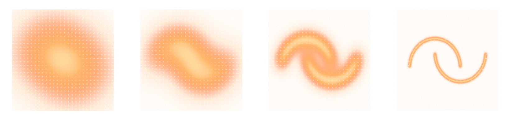
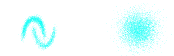
Second Realization: Annealing is everything!
- Even with knowledge of the score, sampling in high number of dimensions is difficult!
- Convolving a target distribution $p$ with a noise kernel, makes $p_\sigma(x) = \int \mathcal{N}(x; x^\prime, \sigma^2) (x^\prime) d x^{\prime}$ it much better behaved
$$\sigma_1 > \sigma_2 > \sigma_3 > \sigma_4 $$
![]()
Score-Based Generative Modeling Song et al. (2021)
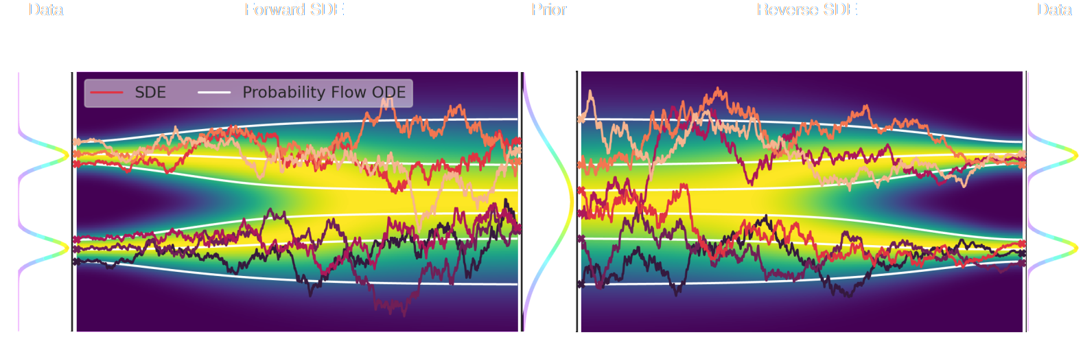
- The SDE defines a marginal distribution $p_t(x)$ as the convolution of the target distribution $p(x)$ with a noise kernel $p_{t|s}(\cdot | x_s)$: $$p_t(x) = \int p(x_s) p_{t|s}(x | x_s) d x_s$$
- For a given forward SDE that evolves $p(x)$ to $p_T(x)$, there exists a reverse SDE that evolves $p_T(x)$ back into $p(x)$. It involves having access to the marginal score $\nabla_x \log_t p(x)$.
Third realization: We do not have access to the marginal posterior score...
- We know the following quantities:
- Annealed likelihood (analytically): $p_\sigma(y | x) = \mathcal{N}(y; \mathbf{A} x, \mathbf{\Sigma} + \sigma^2 \mathbf{I})$
- Annealed prior score (by score matching): $\nabla_x \log p_\sigma(x)$
- But, unfortunately: $\boxed{p_\sigma(x|y) \neq p_\sigma(y|x) \ p_\sigma(x)}$ $\Longrightarrow$ We don't know the marginal posterior score!
- We cannot directly use the reverse SDE/ODE of diffusion models to sample from the posterior. $$\mathrm{d} x = [f(x, t) - g^2(t) \underbrace{\nabla_x \log p_t(x|y)}_{\mbox{unknown}} ] \mathrm{d}t + g(t) \mathrm{d} w$$
Proposed sampling strategy (Remy et al. 2020)
- Even if not equivalent to the marginal posterior score, $\nabla_x \log p_{\sigma^2}(y | x) + \nabla_x \log p_{\sigma^2}(x)$ still
has good properties:
- Tends to an isotropic Gaussian distribution for large $\sigma$
- Corresponds to the target posterior for $\sigma=0$
- If we anneal Langevin or HMC sampling sufficiently slowly (i.e. timescale of change of $\sigma$ is much larger than the timescale of the SDE) we can expect to sample from the target posterior.
High-Dimensional Bayesian Inference for Inverse Problems With Neural Score Estimation
Work in collaboration with:
Benjamin Remy, Zaccharie Ramzi
$\Longrightarrow$ Learn complex priors by Neural Score Estimation and sample from posterior with gradient-based MCMC.
Let's set the stage: Gravitational lensing
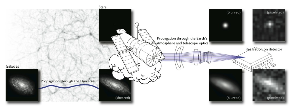
Galaxy shapes as estimators for gravitational shear
$$ e = \gamma + e_i \qquad \mbox{ with } \qquad e_i \sim \mathcal{N}(0, I)$$
- We are trying the measure the ellipticity $e$ of galaxies as an estimator for the gravitational shear $\gamma$
Gravitational Lensing as an Inverse Problem
Shear $\gamma$
![]()
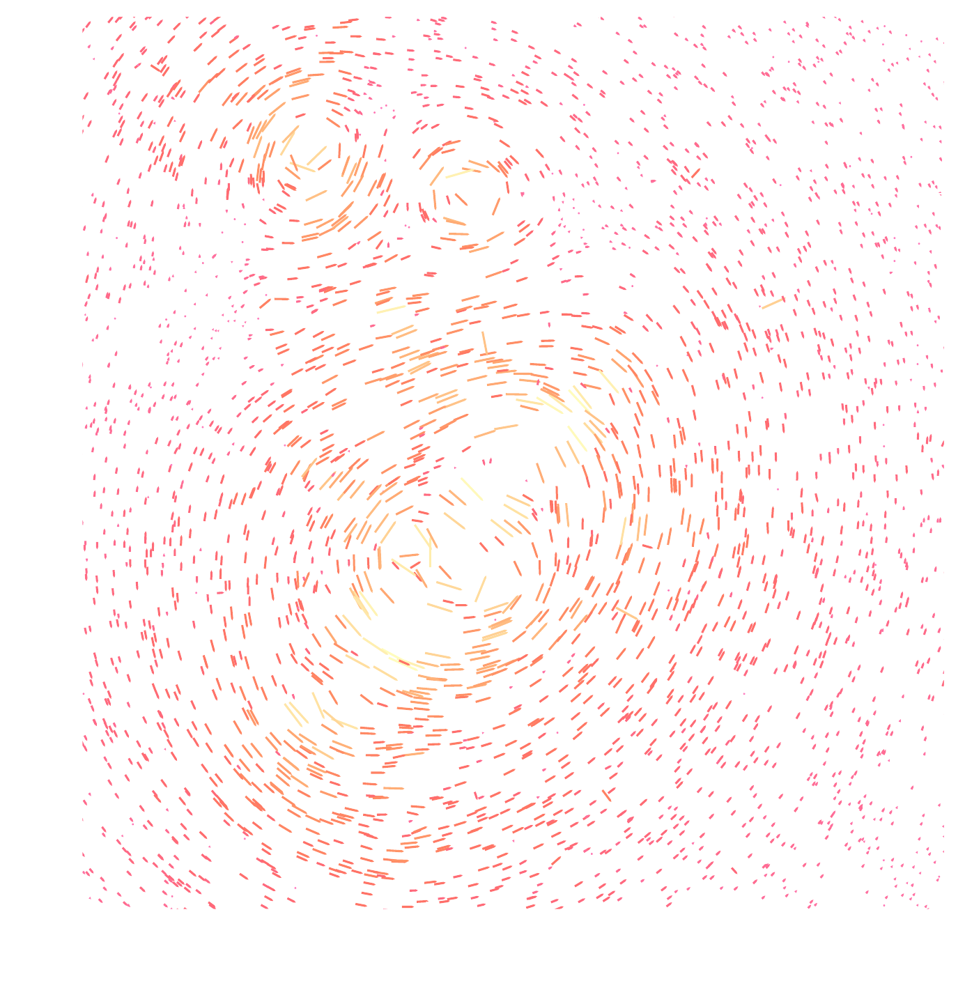
Convergence $\kappa$
![]()
$$\gamma_1 = \frac{1}{2} (\partial_1^2 - \partial_2^2) \ \Psi \quad;\quad \gamma_2 = \partial_1 \partial_2 \ \Psi \quad;\quad \kappa = \frac{1}{2} (\partial_1^2 + \partial_2^2) \ \Psi$$
$$\boxed{\gamma = \mathbf{P} \kappa}$$
Writing down the convergence map log posterior
$$ \log p( \kappa | e) = \underbrace{\log p(e | \kappa)}_{\simeq -\frac{1}{2} \parallel e - P \kappa \parallel_\Sigma^2} + \log p(\kappa) +cst $$- The likelihood term is known analytically, given to us by the physics of gravitational lensing.
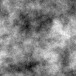
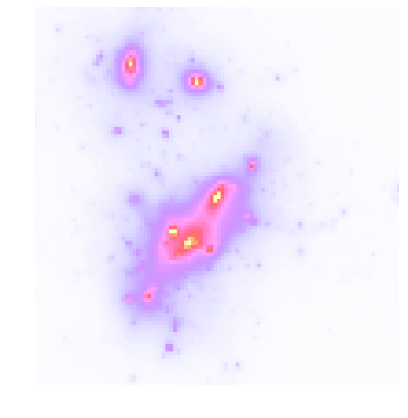
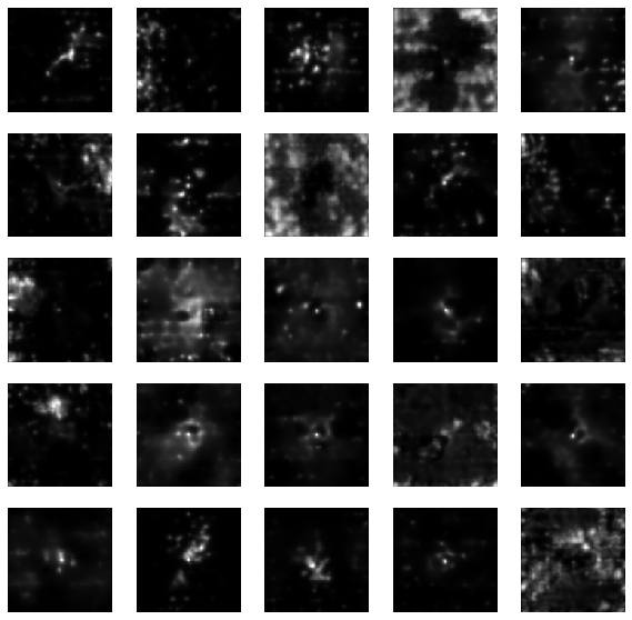
- There is no close form expression for the prior on dark matter maps $\kappa$.
However:- We do have access to samples of full implicit prior through simulations: $X = \{x_0, x_1, \ldots, x_n \}$ with $x_i \sim \mathbb{P}$
![]()
- We do have access to samples of full implicit prior through simulations: $X = \{x_0, x_1, \ldots, x_n \}$ with $x_i \sim \mathbb{P}$
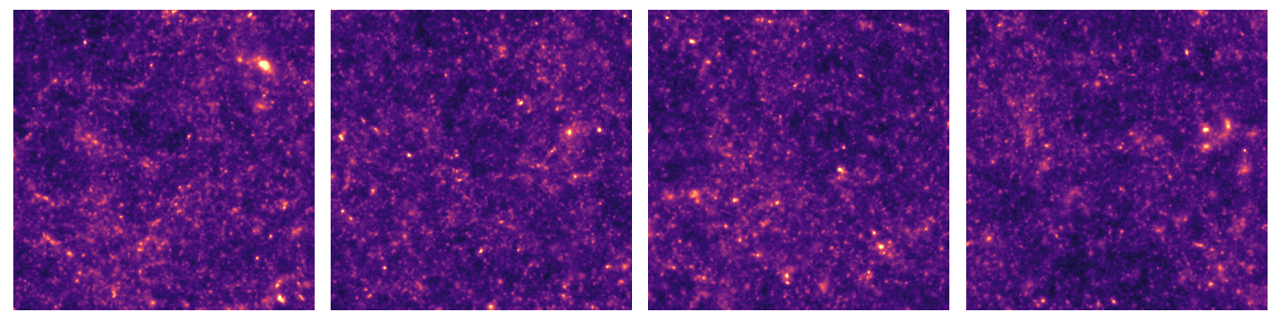
$\Longrightarrow$ Our strategy: Learn the prior from simulation,
and then sample the full posterior.
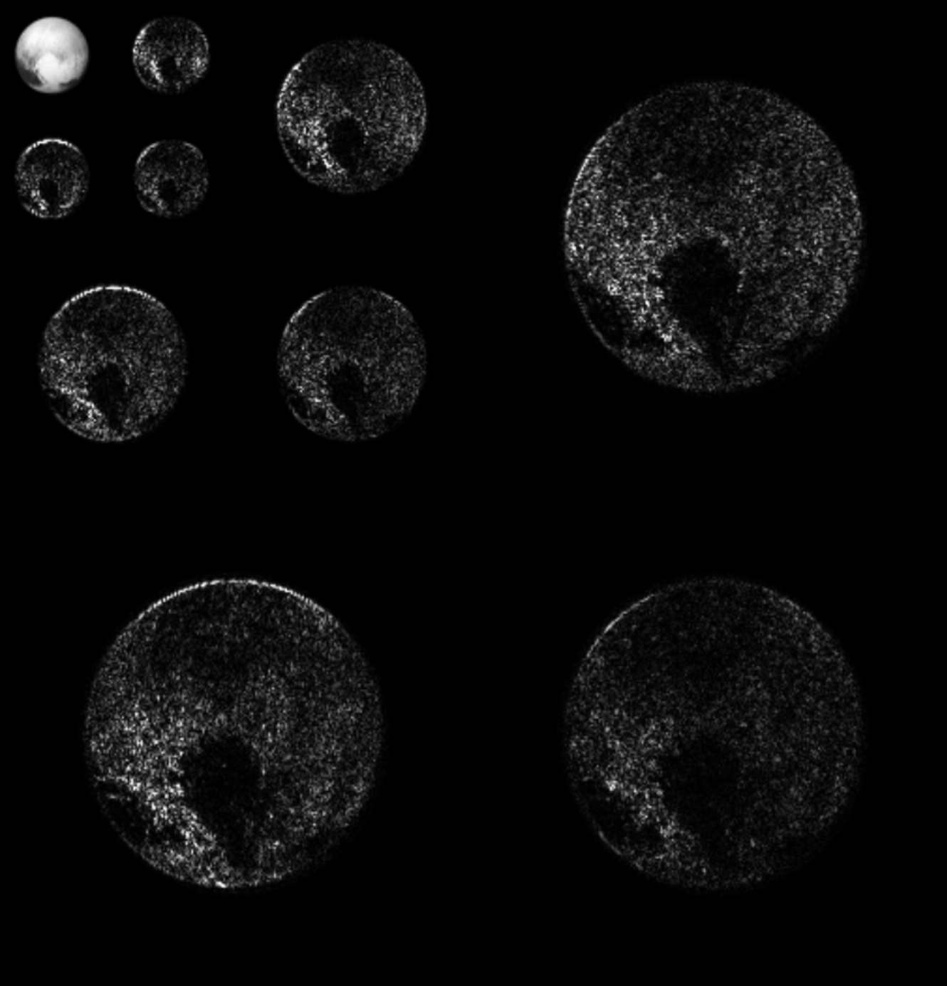
Example of one chain during annealing
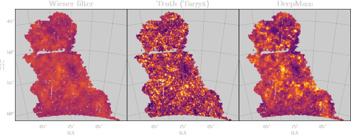
Validating Posterior Sampling under a Gaussian prior
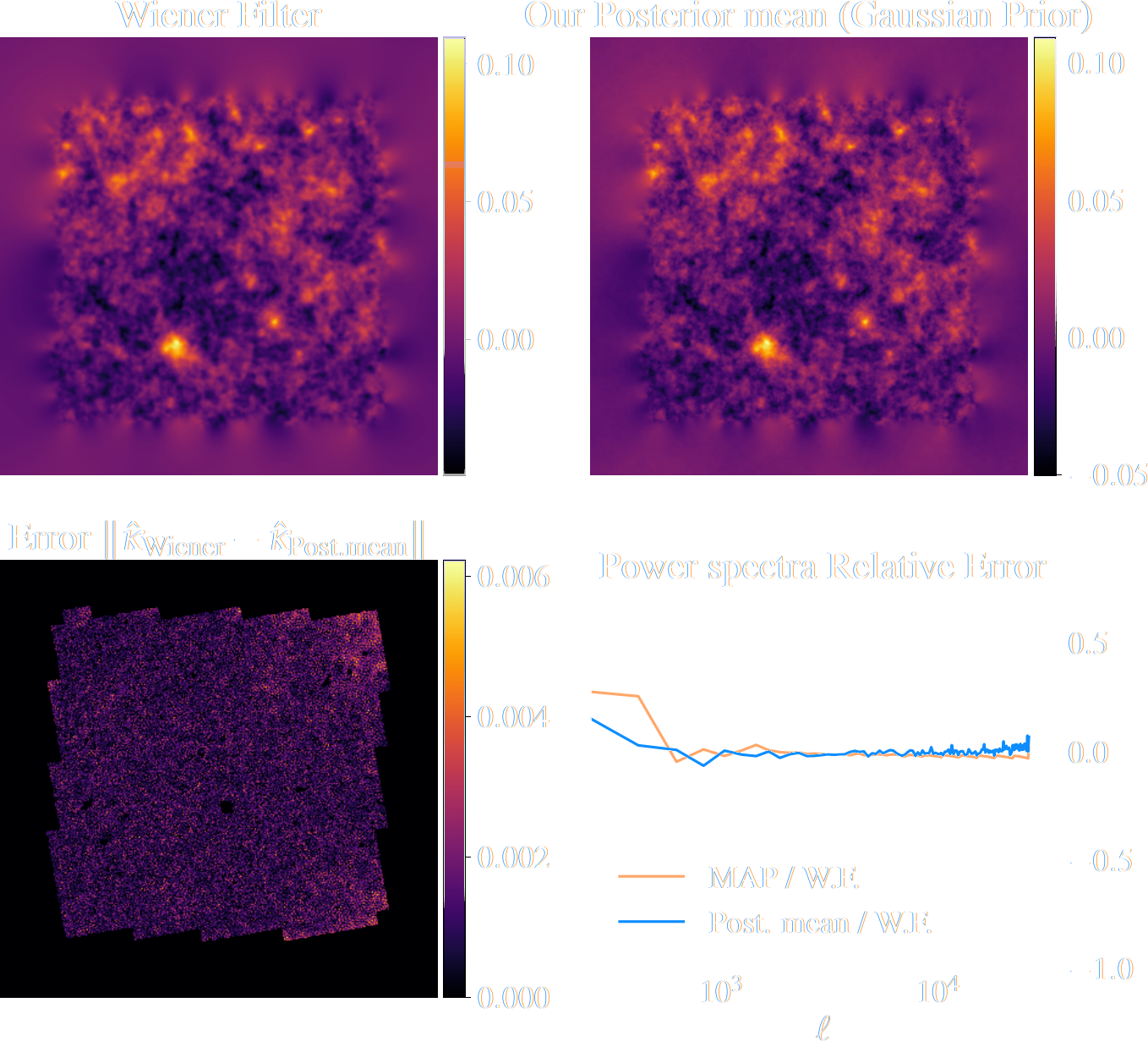
Illustration on $\kappa$-TNG simulations
Remy, Lanusse, et al. (2022) 
True convergence map
Traditional Kaiser-Squires
Wiener Filter
Posterior Mean (ours)
Posterior samples
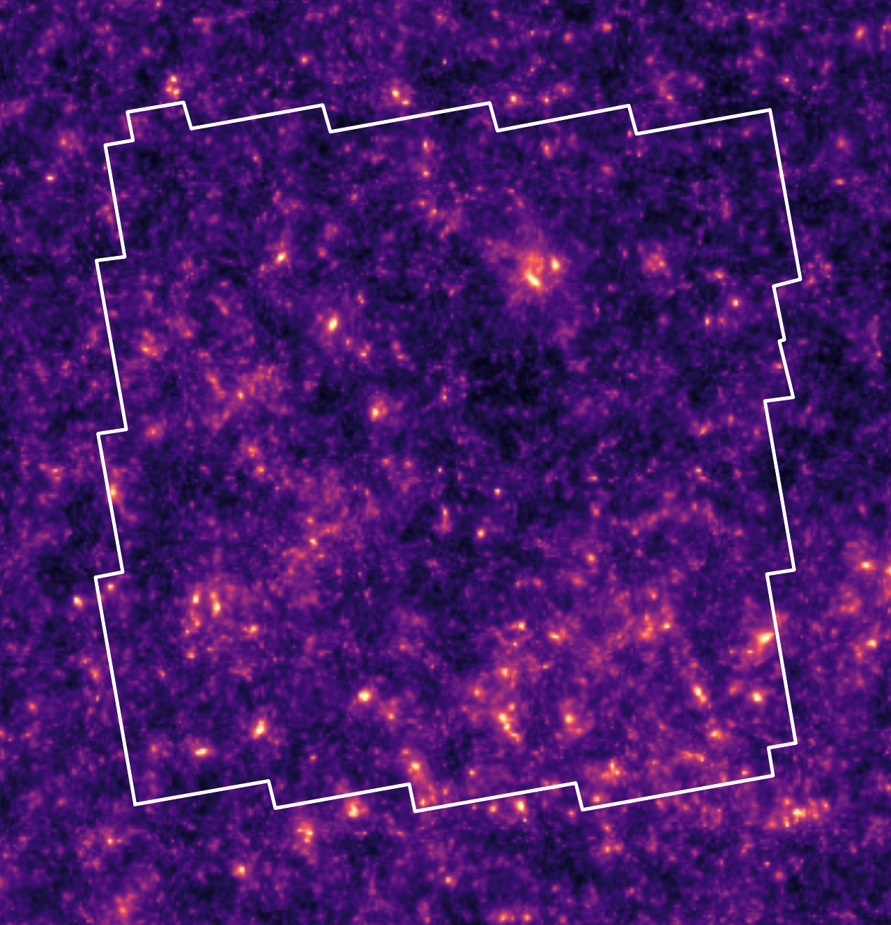
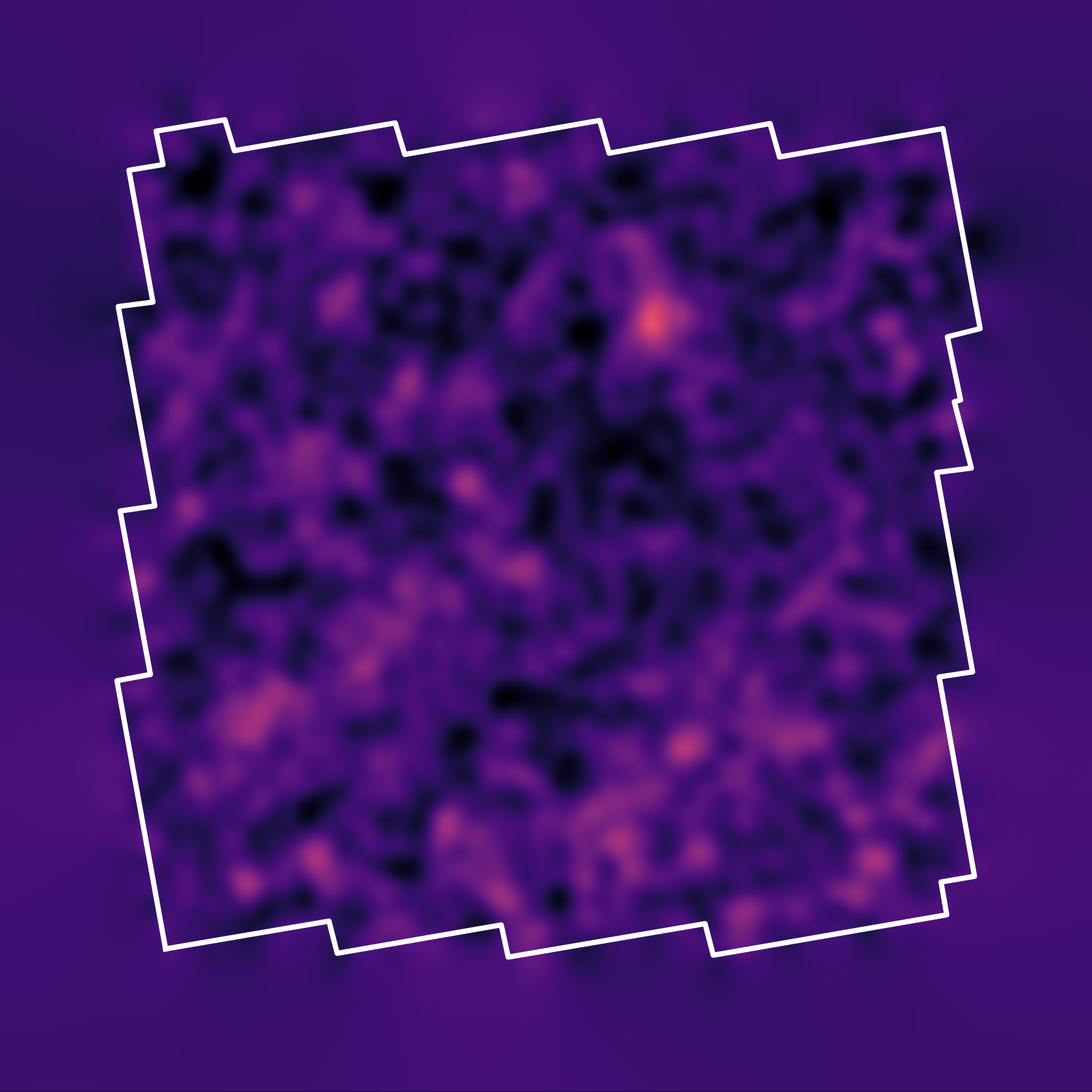
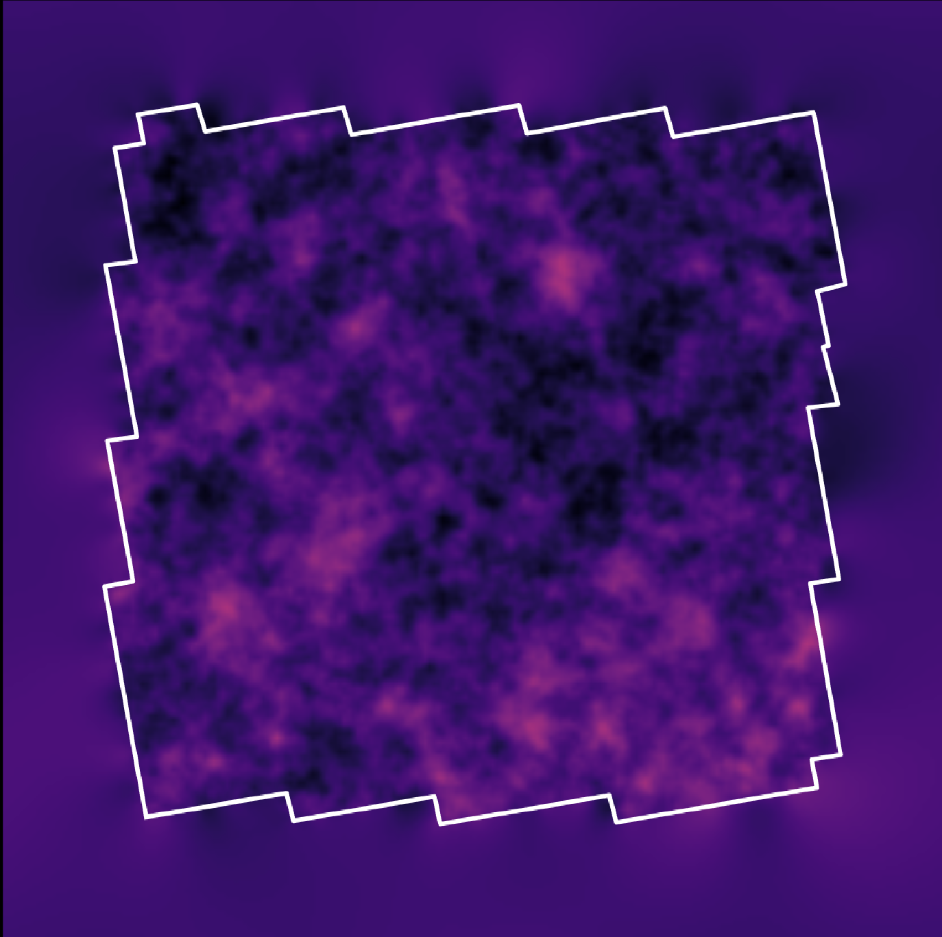
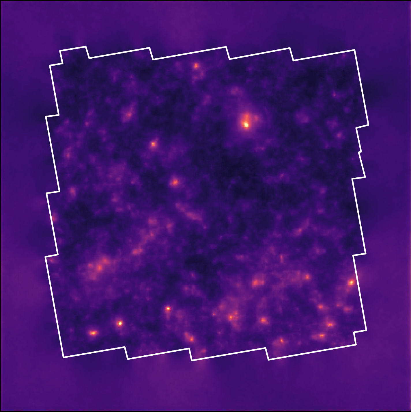
Reconstruction of the HST/ACS COSMOS field
- COSMOS shear data from Schrabback et al. 2010
- Prior learned from $\kappa$-TNG simulation from Osato et al. 2021.
Massey et al. (2007)
![]()
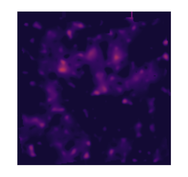
Remy et al. (2022) Posterior mean
![]()
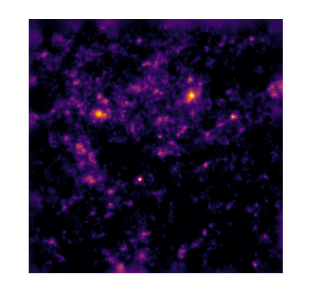
Remy et al. (2022) Posterior samples
![]()
Uncertainty quantification in Magnetic Resonance Imaging (MRI)
Ramzi, Remy, Lanusse et al. 2020 
$$\boxed{y = \mathbf{M} \mathbf{F} x + n}$$
$\Longrightarrow$ We can see which parts of the image are well constrained by data, and which regions are uncertain.
Inference over hybrid physical/data-driven models
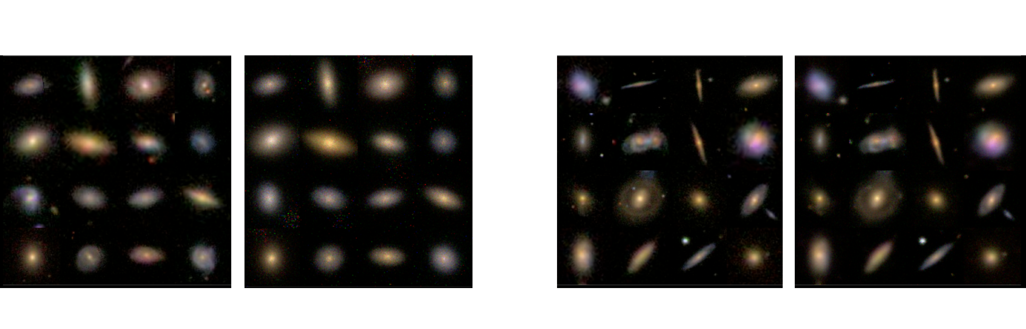
Complications specific to astronomical images: spot the differences!
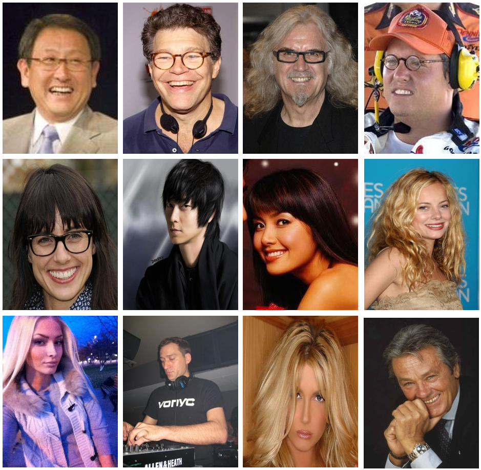
CelebA
HSC PDR-2 wide
- There is noise
- We have a Point Spread Function (instrumental response)
A Physicist's approach: let's build a model
Lanusse et al. (2020) 

$\longrightarrow$
$g_\theta$
$g_\theta$
$\longrightarrow$
PSF
PSF
$\longrightarrow$
Pixelation
Pixelation
$\longrightarrow$
Noise
Noise
Probabilistic model
$$ x \sim ? $$
$$ x \sim \mathcal{N}(z, \Sigma) \quad z \sim ? $$
latent $z$ is a denoised galaxy image
latent $z$ is a denoised galaxy image
$$ x \sim \mathcal{N}( \mathbf{P} z, \Sigma) \quad z \sim ?$$
latent $z$ is a super-resolved and denoised galaxy image
latent $z$ is a super-resolved and denoised galaxy image
$$ x \sim \mathcal{N}( \mathbf{P} (\Pi \ast z), \Sigma) \quad z \sim ? $$
latent $z$ is a deconvolved, super-resolved, and denoised galaxy image
latent $z$ is a deconvolved, super-resolved, and denoised galaxy image
$$ x \sim \mathcal{N}( \mathbf{P} (\Pi \ast g_\theta(z)), \Sigma) \quad z \sim \mathcal{N}(0, \mathbf{I}) $$
latent $z$ is a Gaussian sample
$\theta$ are parameters of the model
latent $z$ is a Gaussian sample
$\theta$ are parameters of the model
$\Longrightarrow$ Decouples the morphology model from the observing conditions.
Bayesian Inference a.k.a. Uncertainty Quantification
The Bayesian view of the problem:
$$ p(z | x ) \propto p_\theta(x | z, \Sigma, \mathbf{\Pi}) p(z)$$
where:
- $p( z | x )$ is the posterior
- $p( x | z )$ is the data likelihood, contains the physics
- $p( z )$ is the prior
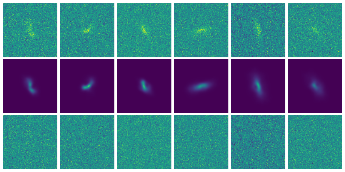
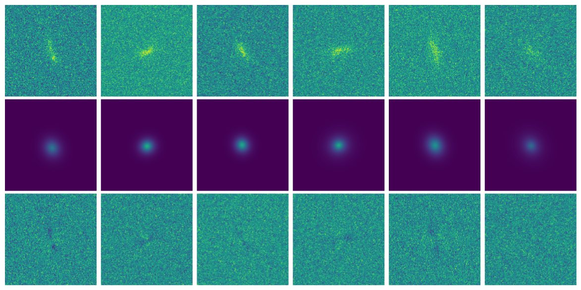
Data
$x_n$
$x_n$
Truth
$x_0$
$x_0$
Posterior samples
$g_\theta(z)$
$g_\theta(z)$
$\mathbf{P} (\Pi \ast g_\theta(z))$
Median
Data residuals
$x_n - \mathbf{P} (\Pi \ast g_\theta(z))$
$x_n - \mathbf{P} (\Pi \ast g_\theta(z))$
Standard Deviation
$\Longrightarrow$ Uncertainties are fully captured by the posterior.
How to train your dragon model
- Training the generative amounts to finding $\theta_\star$ that
maximizes the marginal likelihood of the model:
$$p_\theta(x | \Sigma, \Pi) = \int \mathcal{N}( \Pi \ast g_\theta(z), \Sigma) \ p(z) \ dz$$
$\Longrightarrow$ This is generally intractable
- Efficient training of parameter $\theta$ is made possible by Amortized Variational Inference.
Auto-Encoding Variational Bayes (Kingma & Welling, 2014)
- We introduce a parametric distribution $q_\phi(z | x, \Pi, \Sigma)$ which aims to model the posterior $p_{\theta}(z | x, \Pi, \Sigma)$.
- Working out the KL divergence between these two distributions leads to: $$\log p_\theta(x | \Sigma, \Pi) \quad \geq \quad - \mathbb{D}_{KL}\left( q_\phi(z | x, \Sigma, \Pi) \parallel p(z) \right) \quad + \quad \mathbb{E}_{z \sim q_{\phi}(. | x, \Sigma, \Pi)} \left[ \log p_\theta(x | z, \Sigma, \Pi) \right]$$ $\Longrightarrow$ This is the Evidence Lower-Bound, which is differentiable with respect to $\theta$ and $\phi$.
The famous Variational Auto-Encoder
$$\log p_\theta(x| \Sigma, \Pi ) \geq - \underbrace{\mathbb{D}_{KL}\left( q_\phi(z | x, \Sigma, \Pi) \parallel p(z) \right)}_{\mbox{code regularization}} + \underbrace{\mathbb{E}_{z \sim q_{\phi}(. | x, \Sigma, \Pi)} \left[ \log p_\theta(x | z, \Sigma, \Pi) \right]}_{\mbox{reconstruction error}} $$
Sampling from the model
 Woups... what's going on?
Tradeoff between code regularization and image quality
$$\log p_\theta(x| \Sigma, \Pi ) \geq - \underbrace{\mathbb{D}_{KL}\left( q_\phi(z | x, \Sigma, \Pi) \parallel p(z) \right)}_{\mbox{code regularization}} + \underbrace{\mathbb{E}_{z \sim q_{\phi}(. | x, \Sigma, \Pi)} \left[ \log p_\theta(x | z, \Sigma, \Pi) \right]}_{\mbox{reconstruction error}} $$
Latent space modeling with Normalizing Flows
$\Longrightarrow$ All we need to do is sample from the aggregate posterior of the data instead of sampling from the prior.
Dinh et al. 2016
Normalizing Flows
- Assumes a bijective mapping between data space $x$ and latent space $z$ with prior $p(z)$: $$ z = f_{\theta} ( x ) \qquad \mbox{and} \qquad x = f^{-1}_{\theta}(z)$$
- Admits an explicit likelihood: $$ \log p_\theta(x) = \log p(z) + \log \left| \frac{\partial f_\theta}{\partial x} \right|(x) $$
If you want to code your own Normalizing Flow
This notebook to implement a Normalizing Flow in JAX+Flax+TensorFlow Probability
Flow-VAE samples
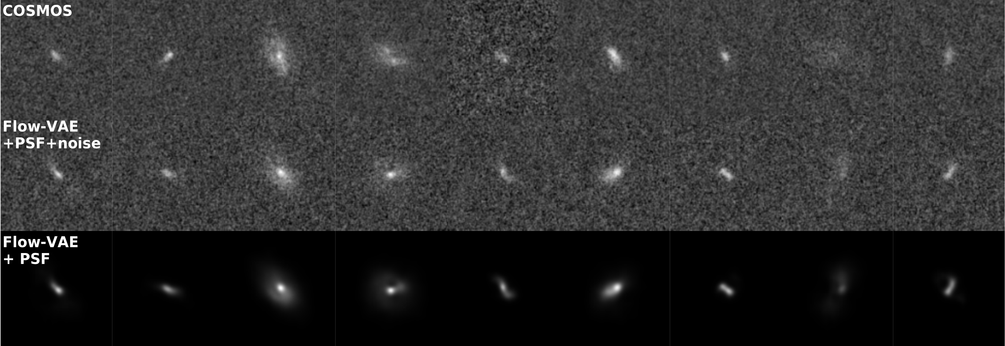
Variational Inference over Hybrid Hierarchical Bayesian Models
Work led by Benjamin Remy
$\Longrightarrow$ Eliminate model bias in shear inference by using data-driven morphology priors.
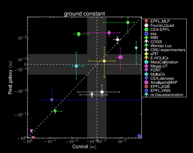
Impact of galaxy morphology on shape measurement
Mandelbaum, et al. (2013), Mandelbaum, et al. (2014)
Let's again think as physicists
$\longrightarrow$
$g_\theta$
$g_\theta$
$\longrightarrow$
shear $\gamma$
shear $\gamma$
$\longrightarrow$
PSF
PSF
$\longrightarrow$
Noise
Noise
Probabilistic model
$$ x \sim \mathcal{N}(\Pi \ast
(g_\theta(z) \otimes \gamma), \Sigma) \quad z \sim \mathcal{N}(0,
\mathbf{I}) $$
latent $z$ are morphological parameters
$\theta$ are global parameters of the model
$\gamma$ are shear parameters
latent $z$ are morphological parameters
$\theta$ are global parameters of the model
$\gamma$ are shear parameters
$\Longrightarrow$ We have a hybrid probabilistic model, with the known physics of lensing and of the instrument, and
learned morphology model.
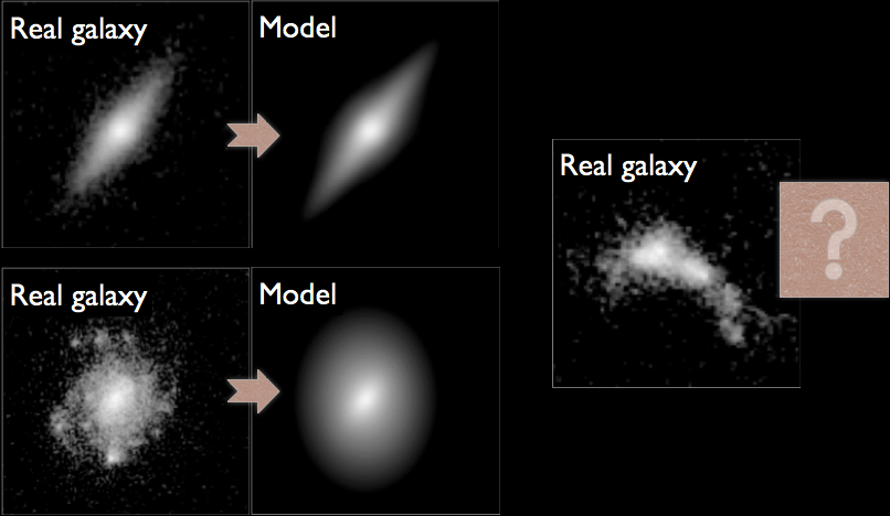
Joint inference using a parametric model for the morphology
Let's assume that $g(z)$ is a sersic model, i.e. $z = \{n, r_\text{hlr}, F, e_1, e_2, s_x, s_y\}$ and
$$g(z) = F \times I_0 \exp \left( -b_n \left[\left( \frac{r}{r_\text{hlr}}\right)^{\frac{1}{n}} -1\right] \right)$$
We need a more realistic model of galaxy morphology
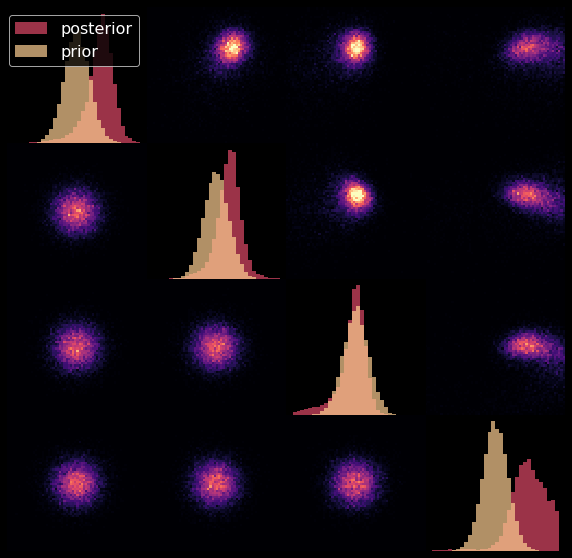
The joint inference of $p(z, \gamma | \mathcal{D})$ leads to a biased posterior...
Marginal shear posterior $p(\gamma|\mathcal{D})$
Maximum a posteriori fit and residuals
Marginal shear posterior $p(\gamma|\mathcal{D})$
Maximum a posteriori fit and residuals
We need a more realistic model of galaxy morphology
Joint inference using a generative model for the morpholgy
Remy, Lanusse, Starck (2022)

Let's use a learned $g_\theta(z)$
The joint inference of $p(z, \gamma | \mathcal{D})$ leads to an unbiased posterior!
Marginal shear posterior $p(\gamma|\mathcal{D})$
Maximum a posteriori fit and residuals
Marginal shear posterior $p(\gamma|\mathcal{D})$
Maximum a posteriori fit and residuals
Conclusion
Conclusion
Merging Deep Learning with Physical Models for Bayesian Inference
$\Longrightarrow$ Makes Bayesian inference possible at scale and with non-trivial models!
- Enables inference in high dimension from numerical simulators.
- By turning implicit physical models into usable explicit distributions.
- Complement known physical models with data-driven components
- Use data-driven generative model as prior for solving inverse problems.
Thank you !