Implicit and Explicit Simulation-Based Bayesian Inference for Cosmology
François Lanusse


slides at eiffl.github.io/talks/Prague2023
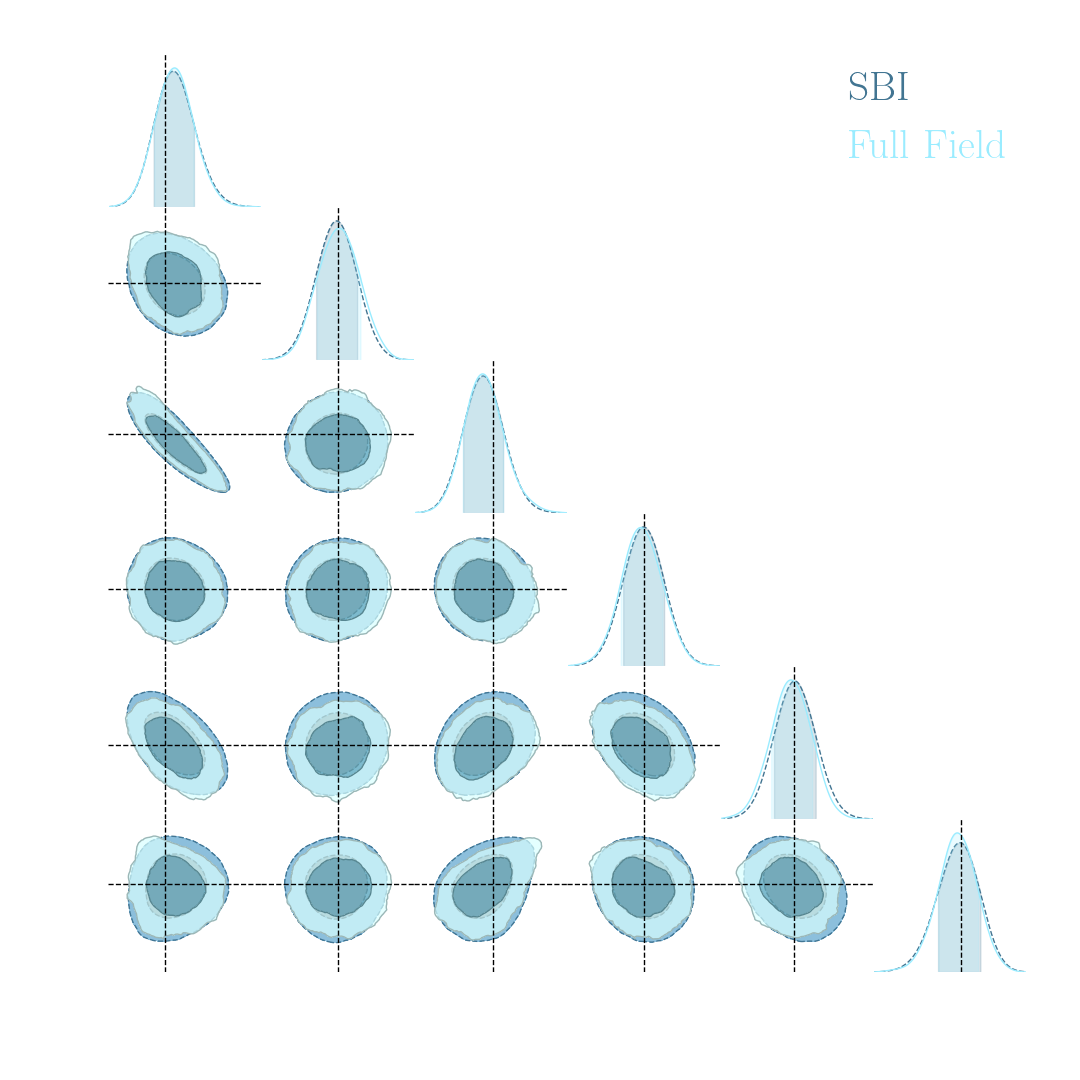
Full-Field Inference
- Instead of analytically evaluating the likelihood of
sub-optimal summary statistics, let us build a model of the full observables.
$\Longrightarrow$ The simulator becomes the physical model. - Each component of the full probabilistic model of the observables is now tractable, but at the cost of a large number of latent variables.
Benefits of a forward modeling approach
- Fully exploits the information content of the data (aka "full field inference").
- Easy to incorporate systematic effects.
- Easy to combine multiple cosmological probes by joint simulations.
(Porqueres et al. 2021)
For now, let's ignore the elephant in the room:
Do we have reliable enough models for the full complexity of the data?
Do we have reliable enough models for the full complexity of the data?
...so why is this not mainstream?
The Challenge of Full-Field Inference
- If we are interested in the likelihood $p(x | \theta)$ we need to marginalize over stochastic latent variables: $$ p(x|\theta) = \int p(x, z | \theta) dz = \int p(x | z, \theta) p(z | \theta) dz $$
- If $x$ is the lensing angular power spectrum, this marginalization can be approximated analytically: $$p(C_\ell | \theta) \simeq \mathcal{N}(C_\ell; C_\ell^{th}, \Sigma)$$
- If $x$ is e.g. a full shear map, this marginalization is analytically intractable.
$\Longrightarrow$ We need to find a tractable way to compute the marginal likelihood $p(x|\theta)$.
How to perform inference over forward simulation models?
- Implicit Inference: Treat the simulator as a black-box with only the ability to sample from the joint distribution
$$(x, \theta) \sim p(x, \theta)$$
a.k.a.
- Simulation-Based Inference (SBI)
- Likelihood-free inference (LFI)
- Approximate Bayesian Computation (ABC)
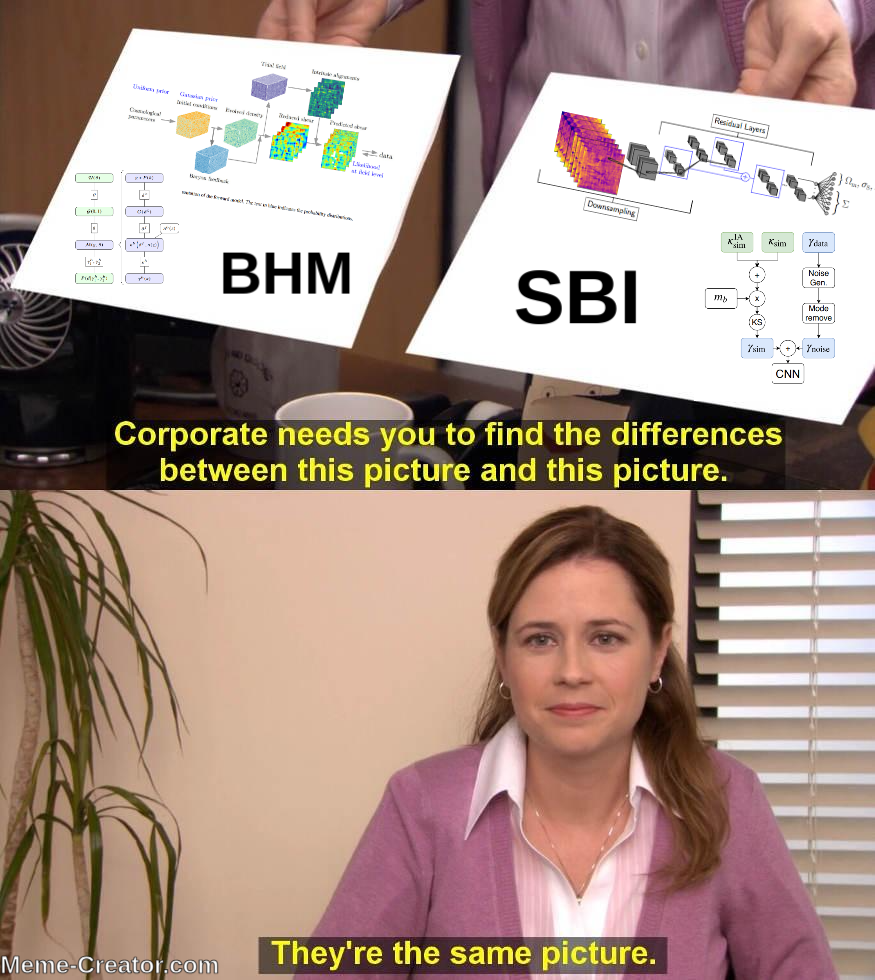
- Explicit Inference: Treat the simulator as a probabilistic model and perform inference over the joint posterior
$$p(\theta, z | x) \propto p(x | z, \theta) p(z, \theta) p(\theta) $$
a.k.a.
- Bayesian Hierarchical Modeling (BHM)
$\Longrightarrow$ For a given simulation model, both methods should converge to the same posterior!
Implicit Inference
The land of Neural Density Estimation
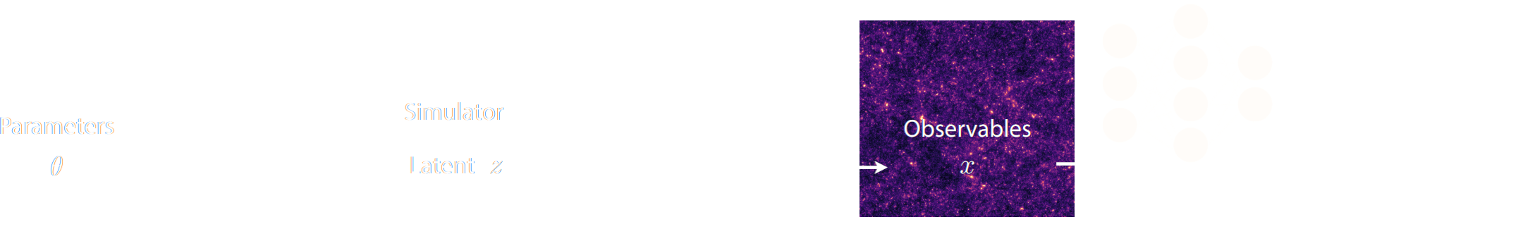
Black-box Simulators Define Implicit Distributions
- A black-box simulator defines $p(x | \theta)$ as an implicit distribution, you can sample from it but you cannot evaluate it.
- Key Idea: Use a parametric distribution model $\mathbb{P}_\varphi$ to approximate the implicit distribution $\mathbb{P}$.

True $\mathbb{P}$

Samples $x_i \sim \mathbb{P}$

Model $\mathbb{P}_\varphi$
- Once trained, you can typically sample from $\mathbb{P}_\varphi$ and/or evaluate the likelihood $p_\varphi(x | \theta)$.
Conditional Density Estimation with Neural Networks
- I assume a forward model of the observations: \begin{equation} p( x ) = p(x | \theta) \ p(\theta) \nonumber \end{equation} All I ask is the ability to sample from the model, to obtain $\mathcal{D} = \{x_i, \theta_i \}_{i\in \mathbb{N}}$
- I am going to assume $q_\phi(\theta | x)$ a parametric conditional density
- Optimize the parameters $\phi$ of $q_{\phi}$ according to \begin{equation} \min\limits_{\phi} \sum\limits_{i} - \log q_{\phi}(\theta_i | x_i) \nonumber \end{equation} In the limit of large number of samples and sufficient flexibility \begin{equation} \boxed{q_{\phi^\ast}(\theta | x) \approx p(\theta | x)} \nonumber \end{equation}
$\Longrightarrow$ One can asymptotically recover the posterior by
optimizing a parametric estimator over
the Bayesian joint distribution
the Bayesian joint distribution
$\Longrightarrow$ One can asymptotically recover the posterior by
optimizing a Deep Neural Network over
a simulated training set.
a simulated training set.
A variety of algorithms
Lueckmann, Boelts, Greenberg, Gonçalves, Macke (2021) 
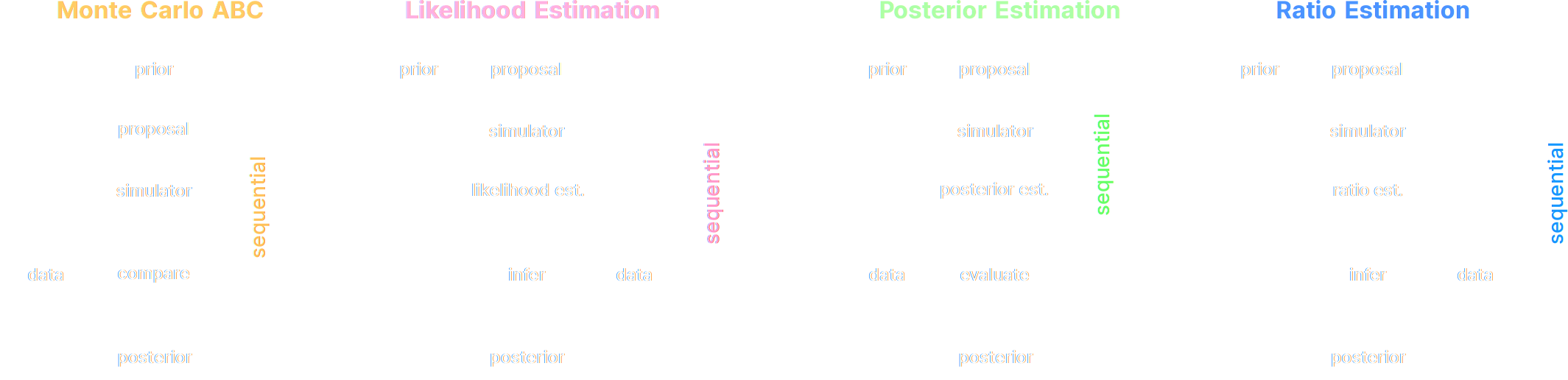
A few important points:
- Amortized inference methods, which estimate $p(\theta | x)$, can greatly speed up posterior estimation once trained.
- Sequential Neural Posterior/Likelihood Estimation methods can actively sample simulations needed to refine the inference.
My Practical Recipe to Apply Neural Density Estimation
A two-steps approach to Likelihood-Free Inference
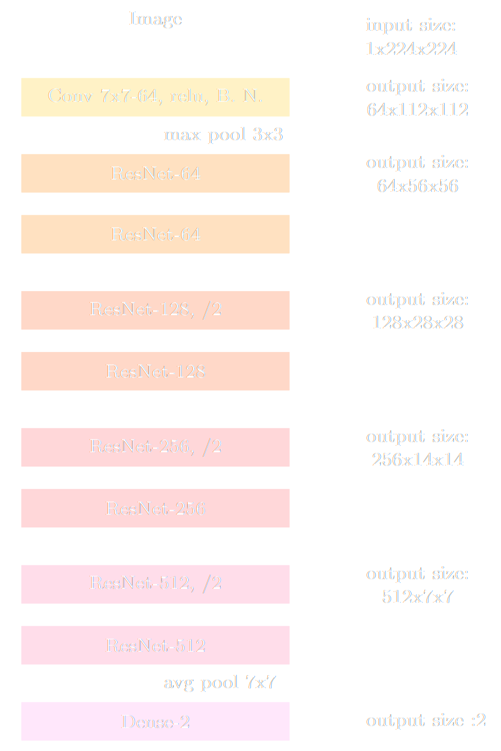
- Step I Automatically learn a optimal low-dimensional summary statistic $$y = f_\varphi(x) $$ typically $y$ will have the same dimensionality as $\theta$.
- Step II: Use Neural Density Estimation in low dimension to either:
- build an estimate $p_\phi$ of the likelihood function $p(y \ | \ \theta)$ (Neural Likelihood Estimation)
- build an estimate $p_\phi$ of the posterior distribution $p(\theta \ | \ y)$ (Neural Posterior Estimation)
Automated Summary Statistics Extraction
- Introduce a parametric function $f_\varphi$ to reduce the dimensionality of the data while preserving information.
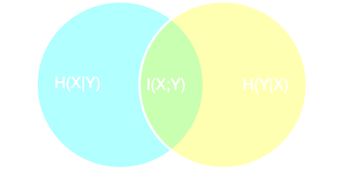
Information-based loss functions
- Summary statistics $y$ is sufficient for $\theta$ if, and only if, $$ I(Y; \Theta) = I(X; \Theta) \Leftrightarrow p(\theta | x ) = p(\theta | y) $$
- Variational Mutual Information Maximization
$$ \mathcal{L} \ = \ \mathbb{E}_{x, \theta} [ \log q_\phi(\theta | f_\varphi(x)) ] \leq I(Y; \Theta) $$
Jeffrey, Alsing, Lanusse (2021)

Example of application: Likelihood-Free parameter inference with DES SV
Jeffrey, Alsing, Lanusse (2021)
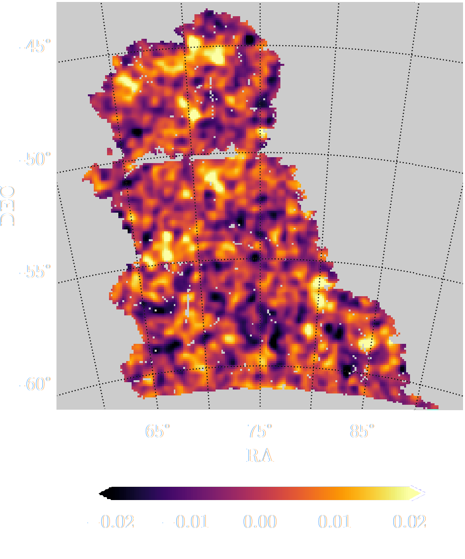
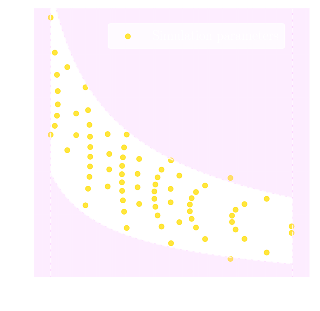
Suite of N-body + raytracing simulations: $\mathcal{D}$
Towards Optimal Full-Field Implicit Inference
by Neural Summarisation and Density Estimation
Work led by Denise Lanzieri and Justine Zeghal


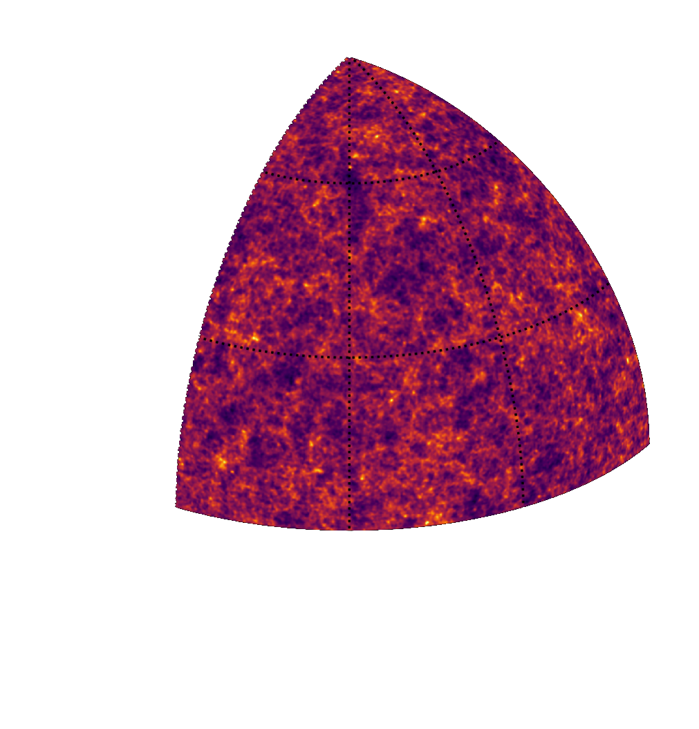
An easy-to-use validation testbed: log-normal lensing simulations

DifferentiableUniverseInitiative/sbi_lens
JAX-based log-normal lensing simulation package
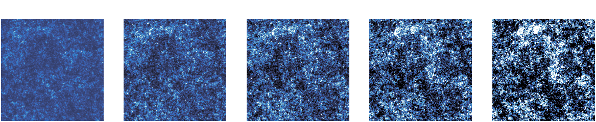
- 10x10 deg$^2$ maps at LSST Y10 quality, conditioning the log-normal shift parameter on $(\Omega_m, \sigma_8, w_0)$
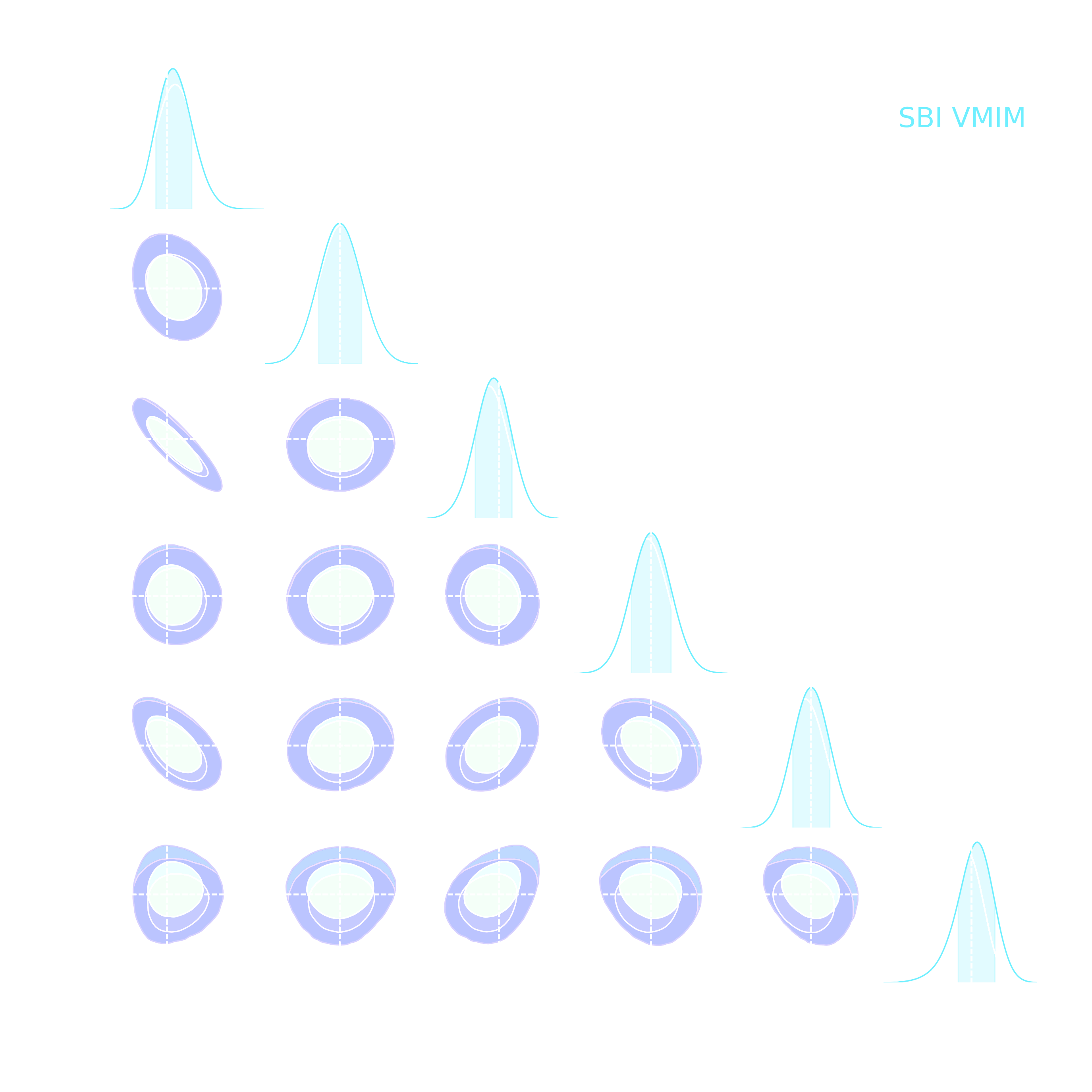
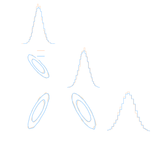
- Infer full-field posterior on cosmology:
- explicitly using an Hamiltonian-Monte Carlo (NUTS) sampler
- implicitly using a learned summary statistics and conditional density estimation.
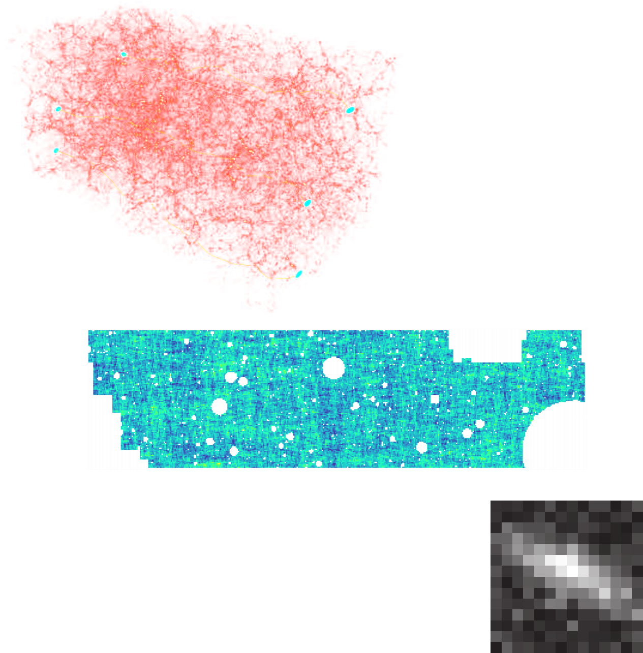
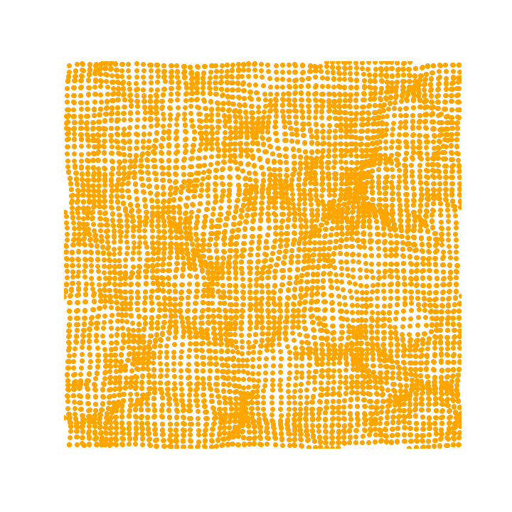
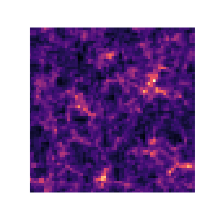
but explicit inference yields intermediate data products
simulated observed data
posterior samples $\kappa = f(z,\theta)$ with $z \sim p(z, \theta | x)$
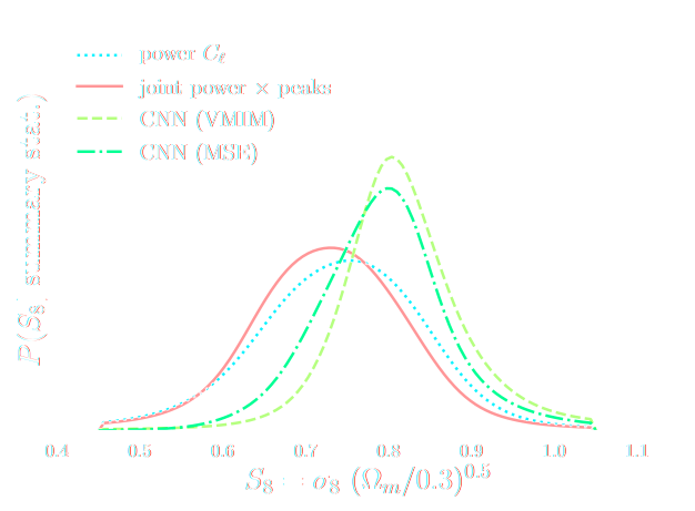
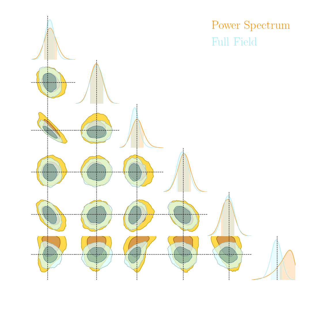
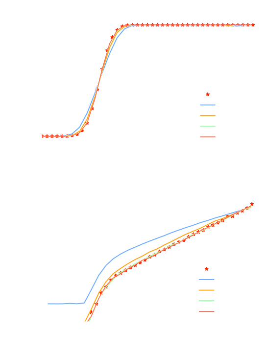
and not all neural compression techniques are equivalent
- Most papers applying neural techniques for inference have used sub-optimal compression techniques, e.g. Mean Square Error $$ \mathcal{L} = || f_\varphi(x) - \theta ||_2^2 $$ $\Longrightarrow$ This is ok, contours will simply be larger than they could be.
- A lot of papers are still relying on assuming a proxy Gaussian likelihoods, i.e. estimating a mean and covariance from
simulations.
$\Longrightarrow$ This is dangerous, can lead to biased contours.
Explicit Inference
Where the JAX things are
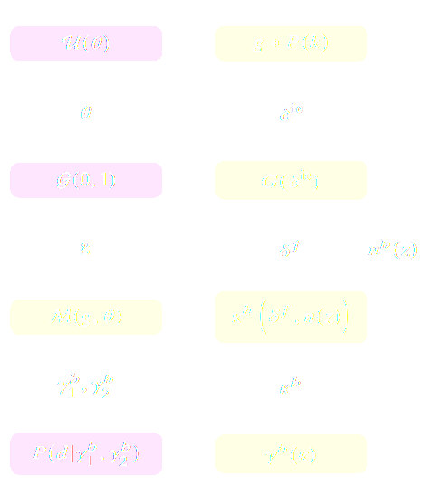
Simulators as Hierarchical Bayesian Models
- If we have access to all latent variables $z$ of the simulator, then the joint log likelihood $p(x | z, \theta)$ is explicit.
- We need to infer the joint posterior $p(\theta, z | x)$ before marginalization to
yield $p(\theta | x) = \int p(\theta, z | x) dz$.
$\Longrightarrow$ Extremely difficult problem as $z$ is typically very high-dimensional. - Necessitates inference strategies with access to gradients of the likelihood. $$\frac{d \log p(x | z, \theta)}{d \theta} \quad ; \quad \frac{d \log p(x | z, \theta)}{d z} $$ For instance: Maximum A Posterior estimation, Hamiltonian Monte-Carlo, Variational Inference.
$\Longrightarrow$ The only hope for explicit cosmological inference is to have fully-differentiable cosmological simulations!
the hammer behind the Deep Learning revolution: Automatic Differentation
- Automatic differentiation allows you to compute analytic derivatives of arbitraty expressions:
If I form the expression $y = a * x + b$, it is separated in fundamental ops: $$ y = u + b \qquad u = a * x $$ then gradients can be obtained by the chain rule: $$\frac{\partial y}{\partial x} = \frac{\partial y}{\partial u} \frac{ \partial u}{\partial x} = 1 \times a = a$$ - This is a fundamental tool in Machine Learning, and autodiff frameworks include TensorFlow and PyTorch.
Enters JAX: NumPy + Autograd + GPU
- JAX follows the NumPy api!
import jax.numpy as np - Arbitrary order derivatives
- Accelerated execution on GPU and TPU
jax-cosmo: Finally a differentiable cosmology library, and it's in JAX!
Campagne, Lanusse, Zuntz et al. (2023)

						import jax.numpy as np
						import jax_cosmo as jc

						# Defining a Cosmology
						cosmo = jc.Planck15()

						# Define a redshift distribution with smail_nz(a, b, z0)
						nz = jc.redshift.smail_nz(1., 2., 1.)

						# Build a lensing tracer with a single redshift bin
						probe = probes.WeakLensing([nz])

						# Compute angular Cls for some ell
						ell = np.logspace(0.1,3)
						cls = angular_cl(cosmo_jax, ell, [probe])
Current main features
- Weak Lensing and Number counts probes
- Eisenstein & Hu (1998) power spectrum + halofit
- Angular $C_\ell$ under Limber approximation
$\Longrightarrow$ 3x2pt DES Y1 capable
let's compute a Fisher matrix
$$F = - \mathbb{E}_{p(x | \theta)}[ H_\theta(\log p(x| \theta)) ] $$
	import jax
	import jax.numpy as np
	import jax_cosmo as jc

	# .... define probes, and load a data vector

	def gaussian_likelihood( theta ):
	  # Build the cosmology for given parameters
	  cosmo = jc.Planck15(Omega_c=theta[0], sigma8=theta[1])

	  # Compute mean and covariance
	  mu, cov = jc.angular_cl.gaussian_cl_covariance_and_mean(cosmo,
														ell, probes)
	  # returns likelihood of data under model
	  return jc.likelihood.gaussian_likelihood(data, mu, cov)

	# Fisher matrix in just one line:
	F = - jax.hessian(gaussian_likelihood)(theta)
- No derivatives were harmed by finite differences in the computation of this Fisher!
- Only a small additional compute time compared to one forward evaluation of the model
Inference becomes fast and scalable
- Current cosmological MCMC chains take days, and typically require access to large computer clusters.
- Gradients of the log posterior are required for modern efficient and scalable inference techniques:
- Variational Inference
- Hamiltonian Monte-Carlo
- In jax-cosmo, we can trivially obtain exact gradients:
def log_posterior( theta ): return gaussian_likelihood( theta ) + log_prior(theta) score = jax.grad(log_posterior)(theta) - On a DES Y1 analysis, we find convergence in 70,000 samples with vanilla HMC, 140,000 with Metropolis-Hastings
DES Y1 posterior, jax-cosmo HMC vs Cobaya MH
(credit: Joe Zuntz)
the Fast Particle-Mesh scheme for N-body simulations
The idea: approximate gravitational forces by estimating densities on a grid.- The numerical scheme:
- Estimate the density of particles on a mesh
=> compute gravitational forces by FFT - Interpolate forces at particle positions
- Update particle velocity and positions, and iterate
- Estimate the density of particles on a mesh
- Fast and simple, at the cost of approximating short range interactions.
$\Longrightarrow$ Only a series of FFTs and interpolations.
introducing FlowPM: Particle-Mesh Simulations in TensorFlow
Modi, Lanusse, Seljak (2020)


																		 import tensorflow as tf
																		 import flowpm
																		 # Defines integration steps
																		 stages = np.linspace(0.1, 1.0, 10, endpoint=True)

																		 initial_conds = flowpm.linear_field(32,       # size of the cube
																											100,       # Physical size
																											ipklin,    # Initial powerspectrum
																											batch_size=16)

																		 # Sample particles and displace them by LPT
																		 state = flowpm.lpt_init(initial_conds, a0=0.1)

																		 # Evolve particles down to z=0
																		 final_state = flowpm.nbody(state, stages, 32)

																		 # Retrieve final density field
																		 final_field = flowpm.cic_paint(tf.zeros_like(initial_conditions),
																										final_state[0])
- Seamless interfacing with deep learning components
Mesh FlowPM: distributed, GPU-accelerated, and automatically differentiable simulations
- We developed a Mesh TensorFlow implementation that can scale on GPU clusters (horovod+NCCL).
- For a $2048^3$ simulation:
- Distributed on 256 NVIDIA V100 GPUs
- Don't hesitate to reach out if you have a use case for model parallelism!
![]()
- Now developing the next generation of these tools in JAX
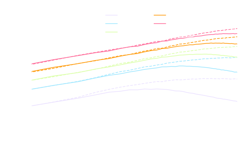
Hybrid physical/neural differential equations
Lanzieri, Lanusse, Starck (2022)

- $\mathbf{x}$ and $\mathbf{v}$ define the position and the velocity of the particles
- $\phi_{PM}$ is the gravitational potential in the mesh
$\to$ We can use this parametrisation to complement the physical ODE with neural networks.
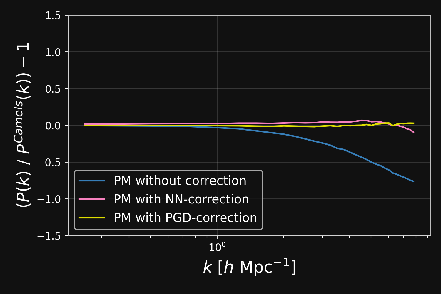
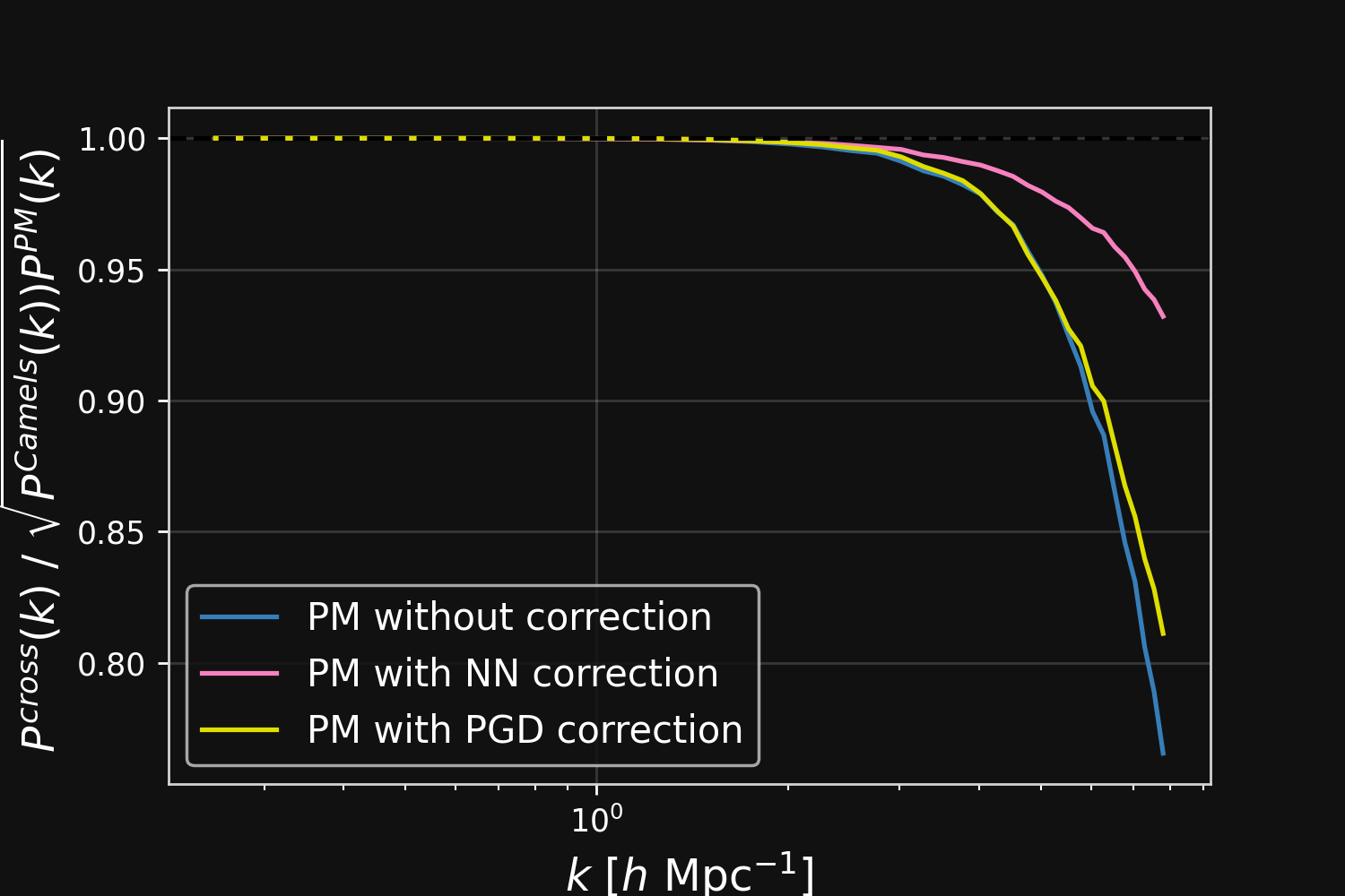
$$F_\theta(\mathbf{x}, a) = \frac{3 \Omega_m}{2} \nabla \left[ \phi_{PM} (\mathbf{x}) \ast \mathcal{F}^{-1} (1 + \color{#996699}{f_\theta(a,|\mathbf{k}|)}) \right] $$
Correction integrated as a Fourier-based isotropic filter $f_{\theta}$ $\to$ incorporates translation and rotation symmetries
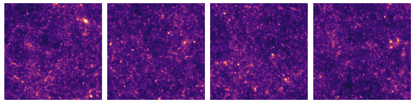
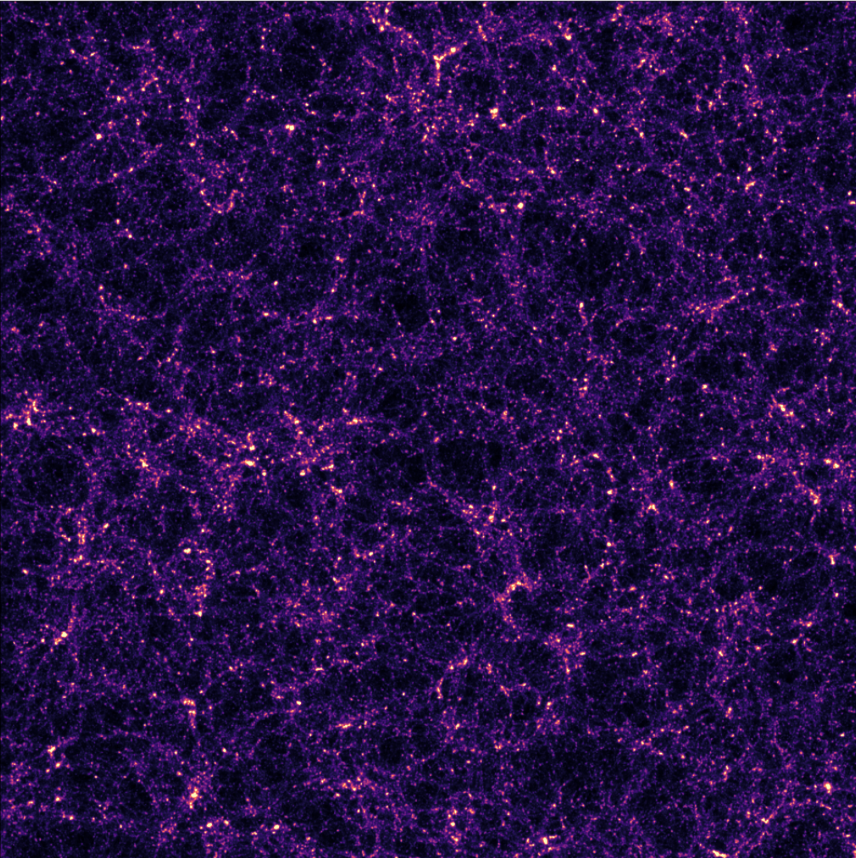
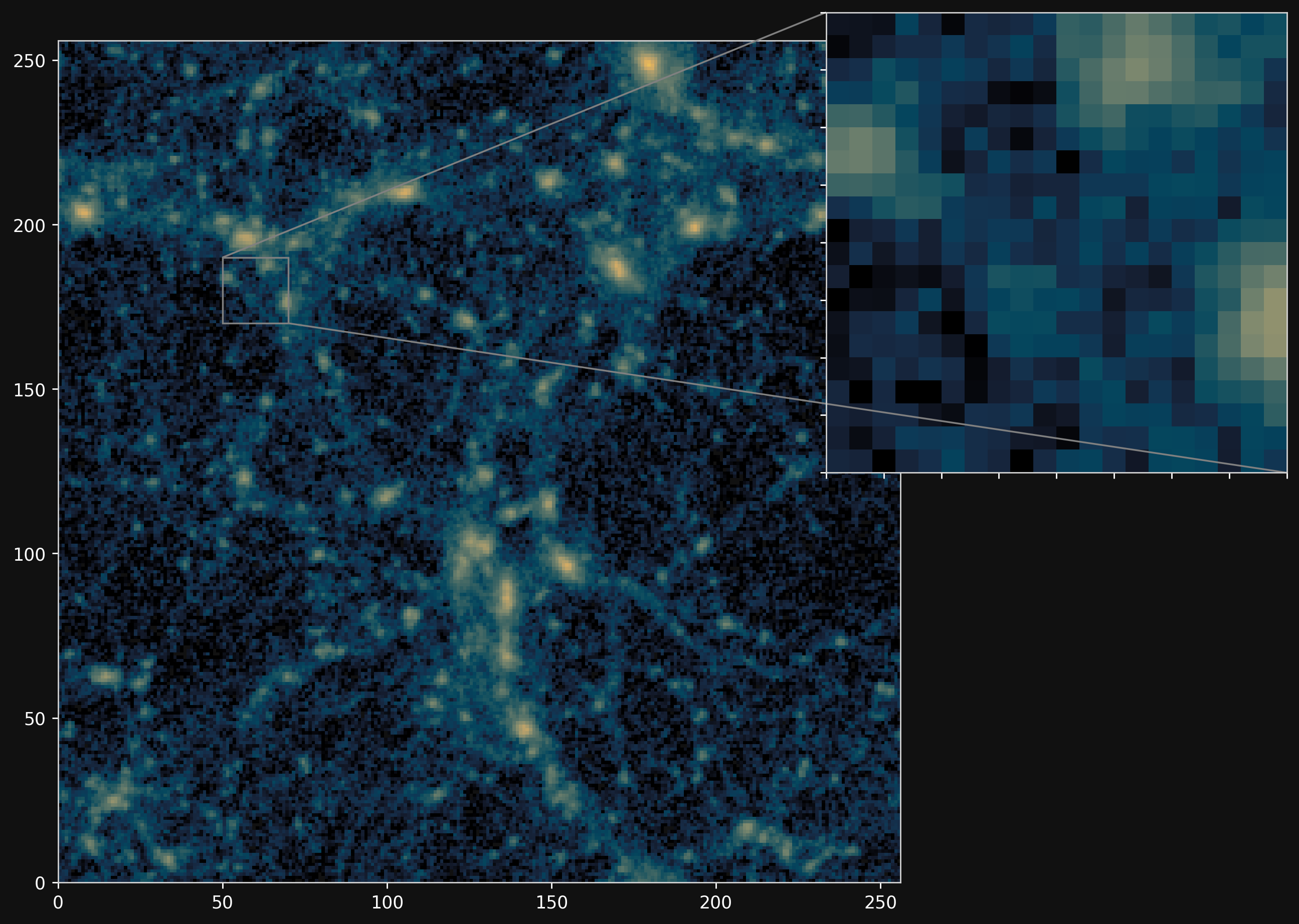
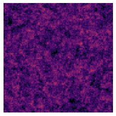
Projections of final density field
Camels simulations
![]()
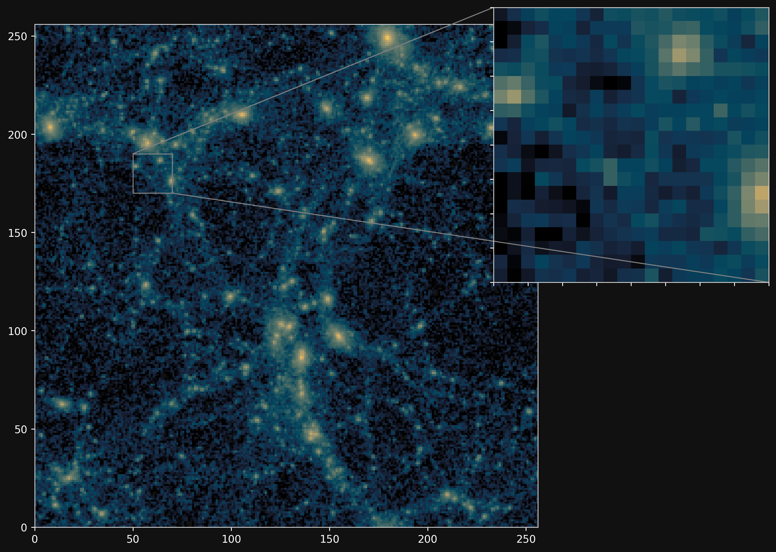
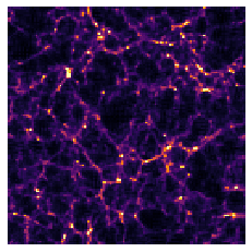
PM simulations
![]()
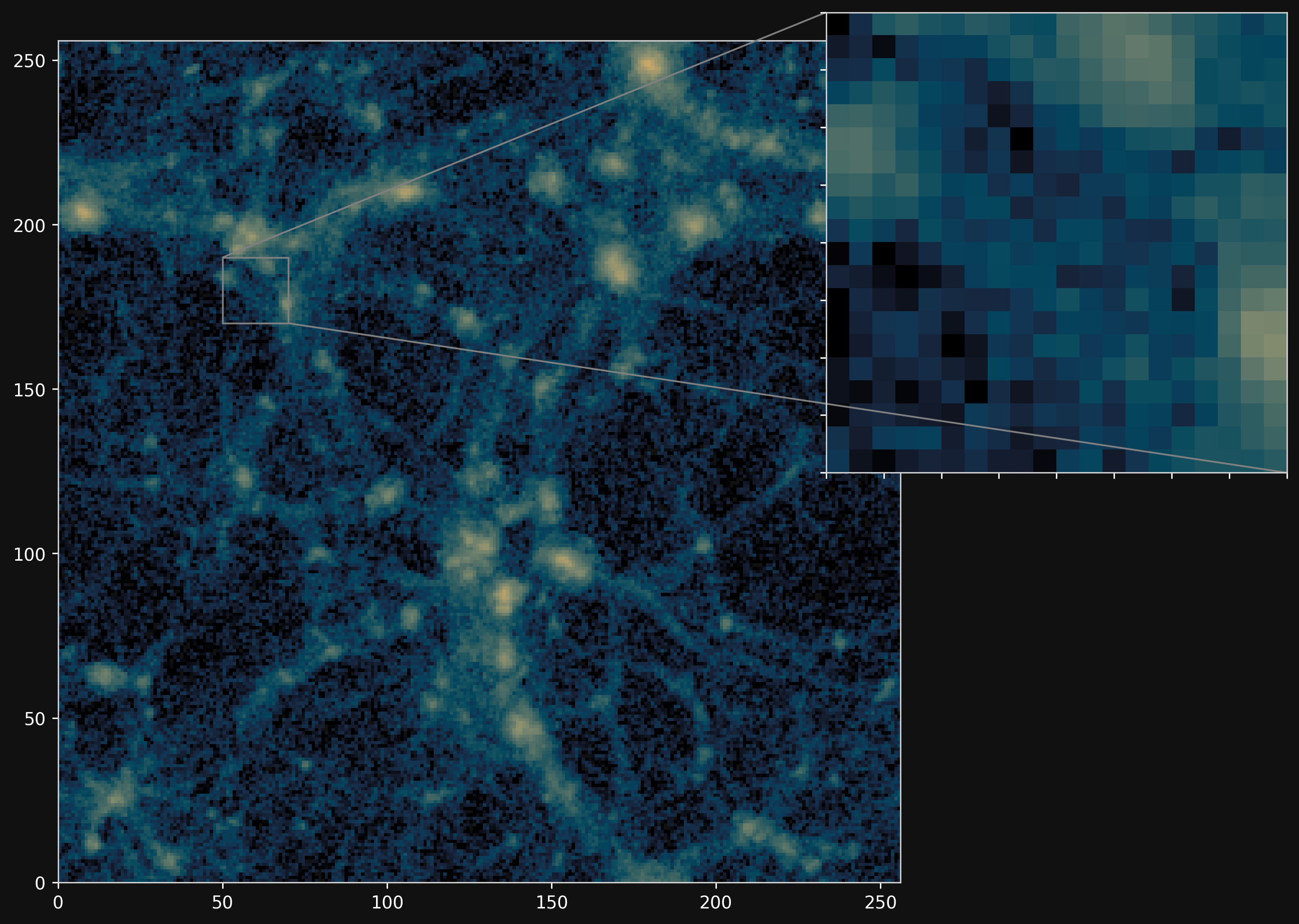
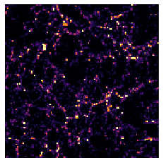
PM+NN correction
![]()
Results
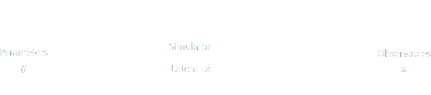
Forward Models in Cosmology
 Linear Field
 Final Dark Matter
 Dark Matter Halos
 Galaxies
$\longrightarrow$
N-body simulations
$\longrightarrow$
Group Finding
algorithms
Group Finding
algorithms
$\longrightarrow$
HOD models
HOD models
Differentiable sampling from Halo Occupation Distributions
Horowitz, Hahn, Lanusse, Modi, Ferraro (2022)

https://github.com/DifferentiableUniverseInitiative/DHOD
- Sampling from a discrete random distribution is classically not a differentiable operation
- Relaxed and reparameterized HOD sampling
- Relaxed Bernoulli distributions for centrals
$$ N_{\rm cen} = \frac{1}{1 + \exp( - (\log(\frac{p}{1 - p}) + \epsilon)/\tau) } \mbox{ with } \epsilon \sim \mathrm{Logistic}(0,1) \;. $$ where $\tau$ is a temperature parameter - Relaxed Binomial distribution for satelittes
$$ N_{\rm sat} \sim \mathrm{Binomial}\left(N, p=\frac{ \left\langle N_{\rm sat}\right\rangle }{N} \right)$$
- Relaxed Bernoulli distributions for centrals
But where are your full-field constraints with Hierarchical Bayesian Inference?
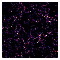
towards reasonable resolution differentiable lensing simulations
Lanzieri, Lanusse, et al. (2023)

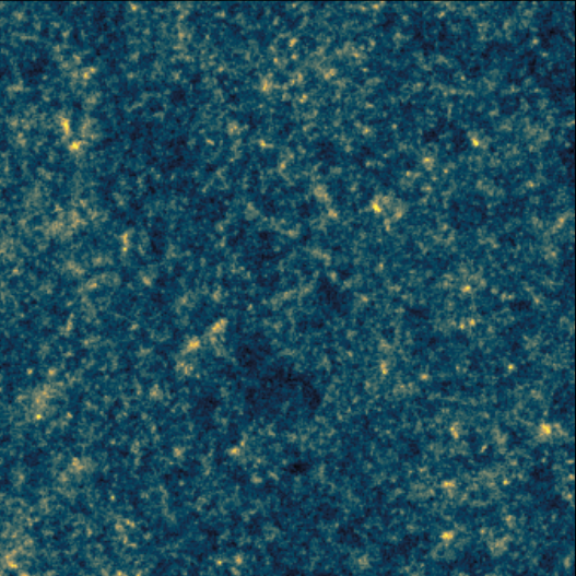
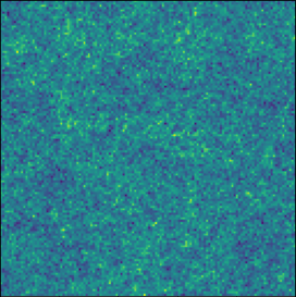
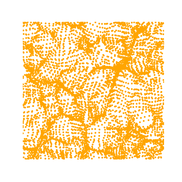
5x5 sq deg^2 convergence field, with sources at z=0.9
FlowPM simulation with 128^3 particles
Conclusion
Conclusion
Methodology for inference over simulators
- A change of paradigm from analytic likelihoods to simulators as physical model.
- State of the art Machine Learning models enable Likelihood-Free Inference over black-box simulators.
- Progress in differentiable simulators and inference methodology paves the way to full inference over probabilistic model.
- Ultimately, promises optimal exploitation of survey data, although the "information gap" against analytic likelihoods in realistic settings remains uncertain.
Thank you!