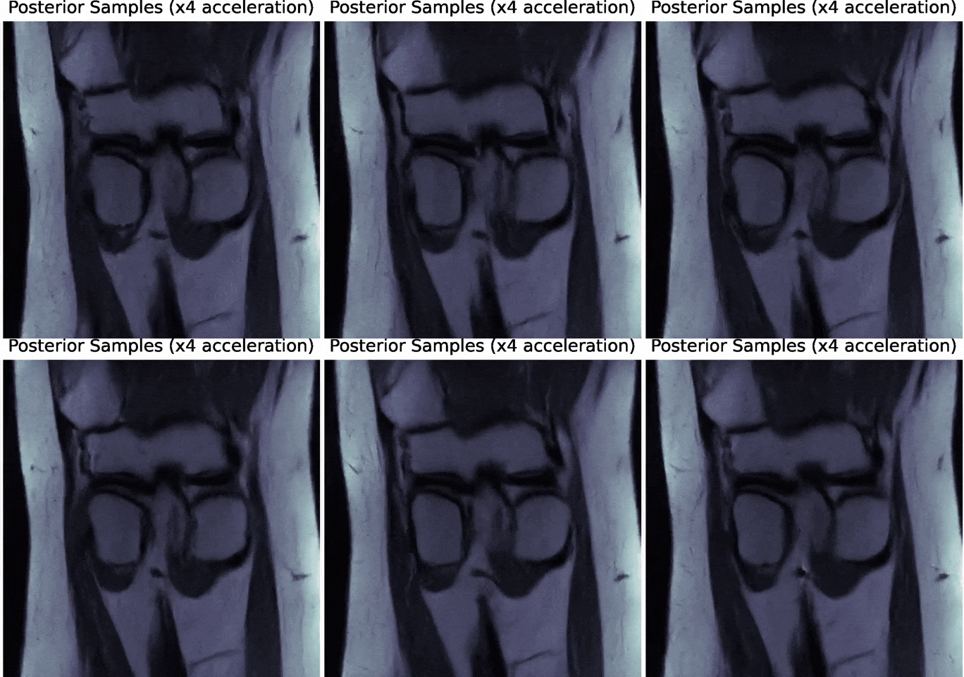
Generative AI for Inverse Problems and Forecasting
AI+Science Summer School, Paris, July 2025
François Lanusse



slides at eiffl.github.io/talks/Paris2025
Learning Objectives & Program

$+ p(x) =$

- First Hour: Combining Physical Models and Generative Modeling
- Understanding the limits of black-box deep learning
- Taking a Bayesian point of view on inverse problems
- Using generative models to capture implicit distributions
- Applications in astrophysics: mapping the invisible dark matter
- Second Hour: Practical Work: Conditional Forecasting for Heliophysics
- Compare deterministic vs stochastic forecasting methods
- Implement guidance with explicit likelihood on a diffusion model
A Motivating Example: Image Deconvolution
$ y = P \ast x + n $
Observed $y$
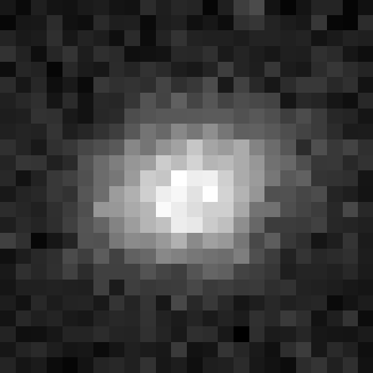
Ground-Based Telescope
$f_\theta$
some deep Convolutional Neural Network
Unknown $x$
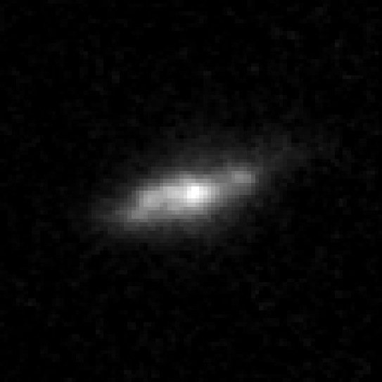
Hubble Space Telescope
- A standard approach would be to train a neural network $f_\theta$ to estimate $x$ given $y$.
- Step I: Assemble from data or simulations a training set of images $$\mathcal{D} = \{(x_0, y_0), (x_1, y_1), \ldots, (x_N, y_N) \}$$ $\Longrightarrow$ the dataset contains hardcoded assumptions about PSF $P$ noise $n$, and galaxy morphology $x$.
- Step II: Train the neural network $f_\theta$ under a regression loss of the type: $$ \mathcal{L} = \sum_{i=0}^N \parallel x_i - f_\theta(y_i)\parallel^2 $$
$$ y $$
$$f_\theta$$
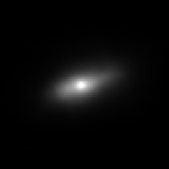 $$f_\theta(y)$$
$$ \mbox{True } x $$
$\Longrightarrow$Why is the network output different from the truth? If it's
not the truth, then what is $f_\theta(y)$?
A neural network will try to answer
the question you ask.
Let's try to understand the neural network output by looking at the loss function
$$ \mathcal{L} = \sum_{(x_i, y_i) \in \mathcal{D}} \parallel x_i - f_\theta(y_i)\parallel^2 \quad \simeq \quad \int \parallel x - f_\theta(y) \parallel^2 \ p(x,y) \ dx dy $$$$\Longrightarrow \int \left[ \int \parallel x -
f_\theta(y) \parallel^2 \ p(x|y) \ dx \right] p(y) dy $$
$\mathcal{L}$ minimized when $f_{\theta^\star}(y) = \int x \ p(x|y) \ dx $, i.e.
when $f_{\theta^\star}(x)$ is predicting the mean of $p(x|y)$.
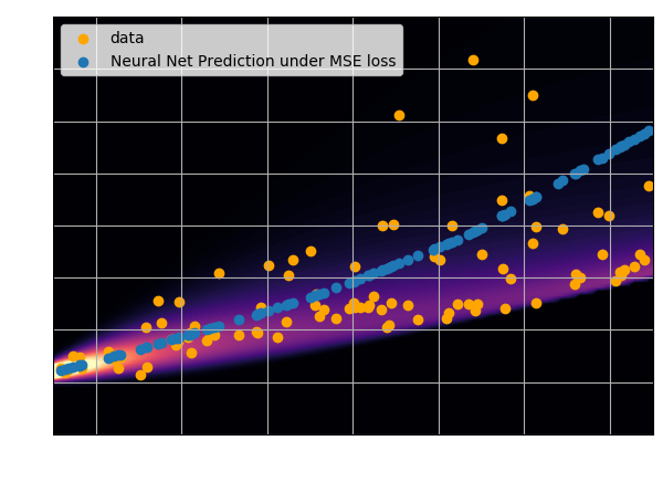
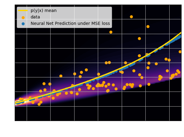
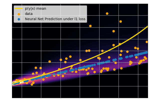
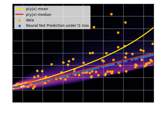
- Using an $\ell_2$ loss learns the mean of the $p(x | y)$
- Using an $\ell_1$ loss learns the median of $p(x|y)$
- In general, training a neural network for
regression doesn't
achieve de mode of the distribution.
Check this blogpost to learn more about that.
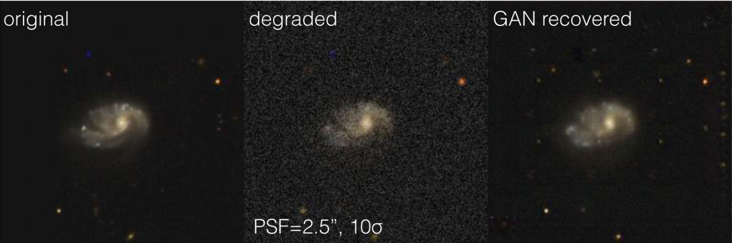
Example: GalaxyGAN (Schawinski et al. 2017)
Linear inverse problems
$\boxed{y = \mathbf{A}x + n}$$\mathbf{A}$ is known and encodes our physical understanding of the problem.
$\Longrightarrow$ When non-invertible or ill-conditioned, the inverse problem is ill-posed with no unique solution $x$
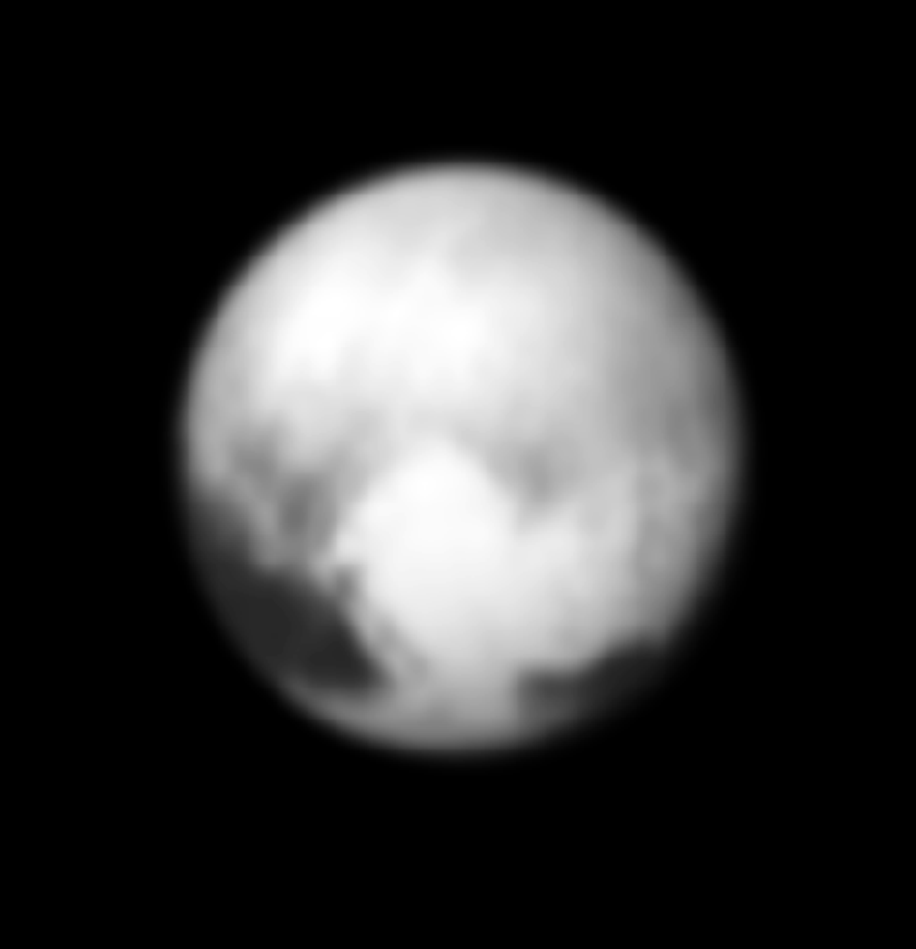 Deconvolution
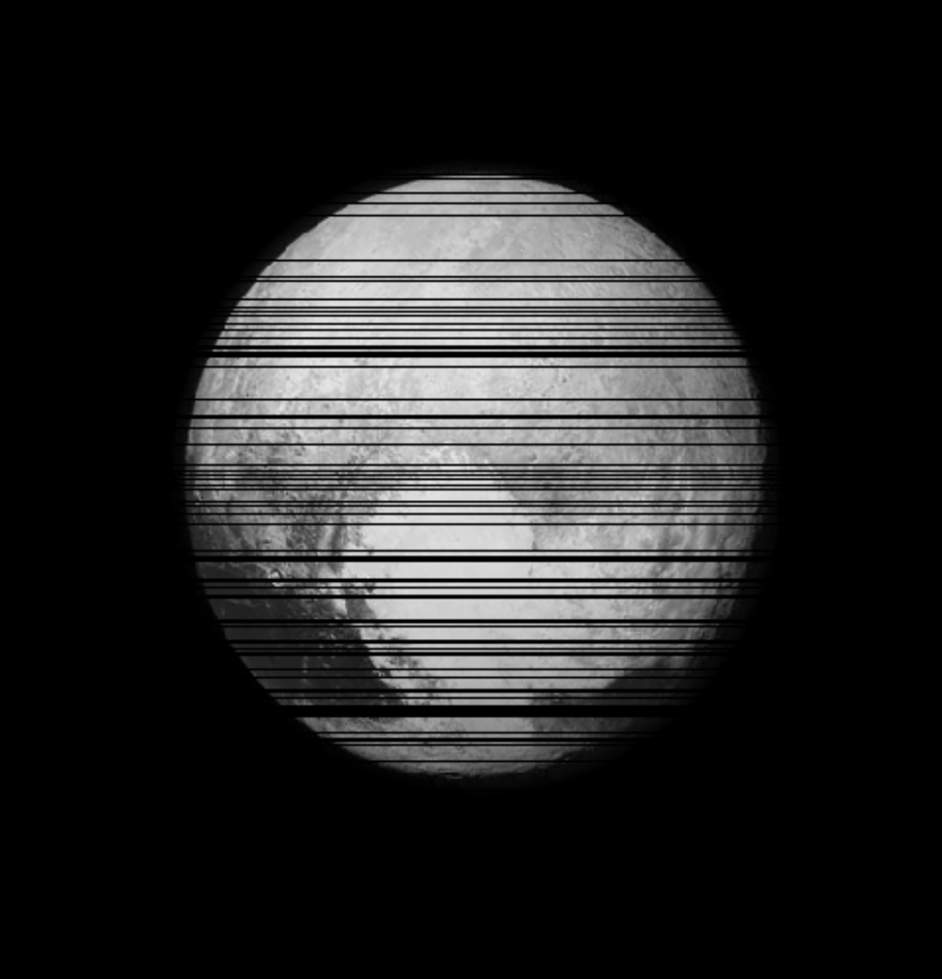 Inpainting
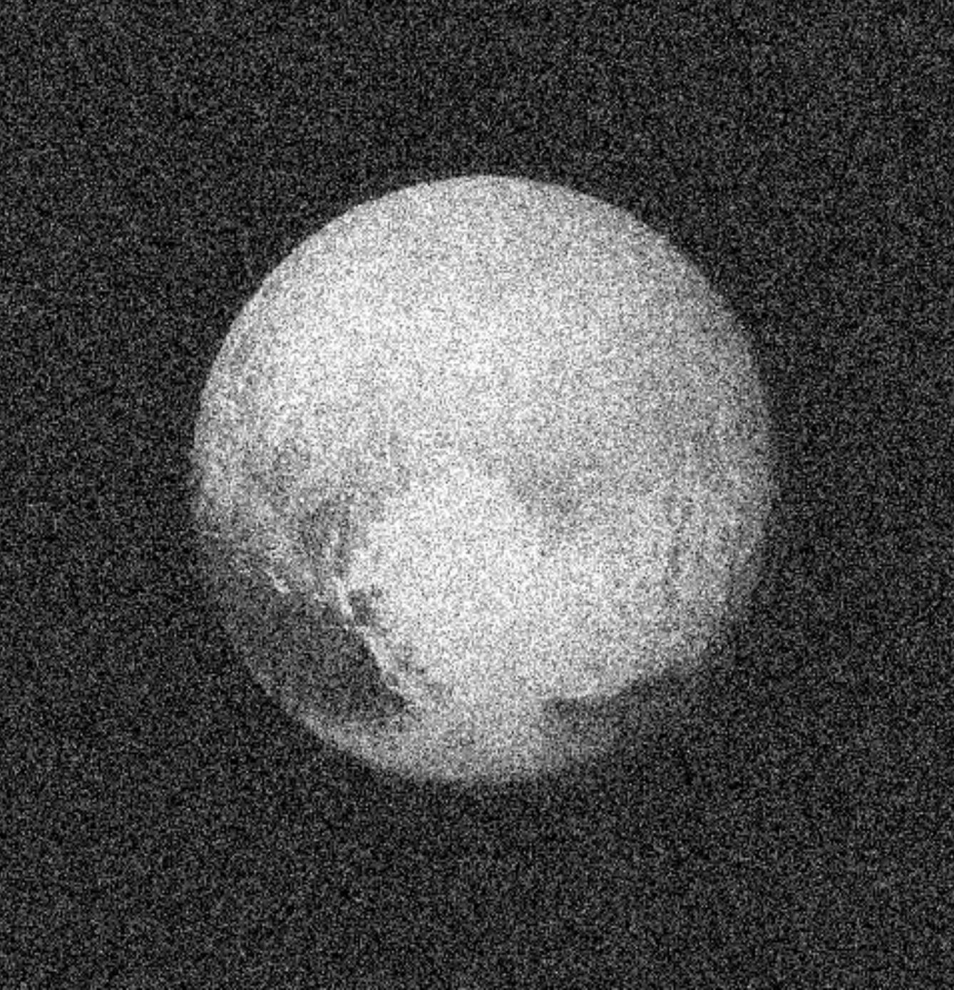 Denoising
A Bayesian view of the problem
$\boxed{y = \mathbf{A}x + n}$
$$ p(x | y) \propto p(y | x) \ p(x) $$
- $p(y | x)$ is the data likelihood, which contains the
physics
- $p(x)$ is our prior knowledge on the solution.
With these concepts in hand, we can for instance estimate the Maximum A Posteriori solution:
$$\hat{x} = \arg\max\limits_x \ \log p(y \ | \ x) + \log p(x)$$ For instance, if $n$ is Gaussian, $\hat{x} = \arg\max\limits_x \ - \frac{1}{2} \parallel y - \mathbf{A} x \parallel_{\mathbf{\Sigma}}^2 + \log p(x)$
$$\hat{x} = \arg\max\limits_x \ \log p(y \ | \ x) + \log p(x)$$ For instance, if $n$ is Gaussian, $\hat{x} = \arg\max\limits_x \ - \frac{1}{2} \parallel y - \mathbf{A} x \parallel_{\mathbf{\Sigma}}^2 + \log p(x)$
Or, we can aim to sample from the full posterior distribution by MCMC techniques.
How do you choose the prior ?
Classical examples of signal priors
Sparse
![]()
$$ \log p(x) = \parallel \mathbf{W} x \parallel_1 $$
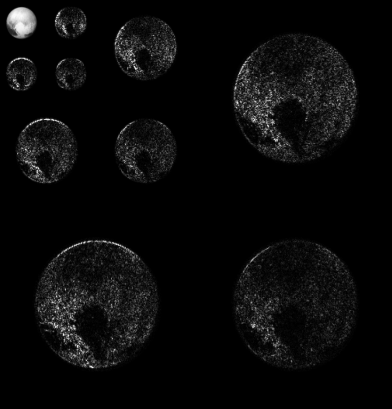
$$ \log p(x) = \parallel \mathbf{W} x \parallel_1 $$
Gaussian
![]() $$ \log p(x) = x^t \mathbf{\Sigma^{-1}} x $$
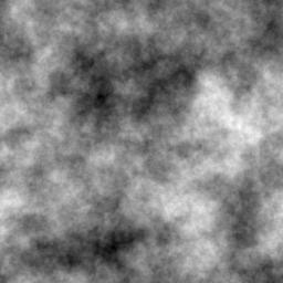 $$ \log p(x) = x^t \mathbf{\Sigma^{-1}} x $$
Total Variation
![]() $$ \log p(x) = \parallel \nabla x \parallel_1 $$
But what about this?
Maybe we can learn priors from the data!
- Generative modeling aims to learn an implicit distribution $\mathbb{P}$ from which the training set $X = \{x_0, x_1, \ldots, x_n \}$ is drawn.
- Usually, this means building a parametric model $\mathbb{P}_\theta$ that tries to be close to $\mathbb{P}$.

True $\mathbb{P}$

Samples $x_i \sim \mathbb{P}$

Model $\mathbb{P}_\theta$
- Once trained, you can typically sample from $\mathbb{P}_\theta$ and/or evaluate the probability $p_\theta(x)$.
Why are these generative models useful?
Implicit distributions are everywhere!
Case I: Examples from data, no accurate physical model
![]()
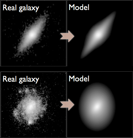
Mandelbaum et al. 2014
Case II: Physical model only available as a simulator
![]()
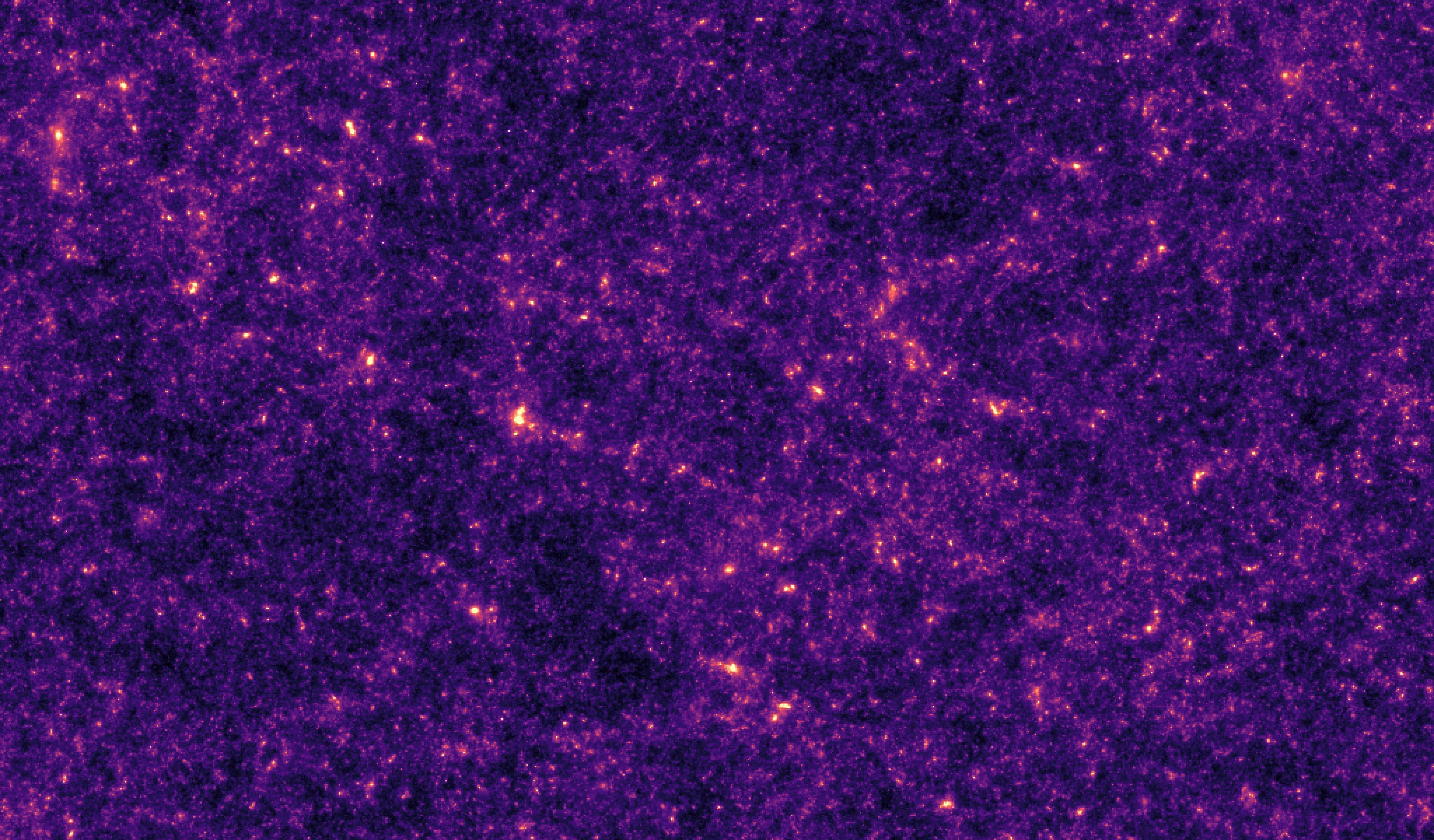
Osato et al. 2020
$\Longrightarrow$ Generative models will enable Bayesian
inference in cases where
implicit distributions are involved, by providing a tractable $p_\theta(x)$.
The evolution of generative models
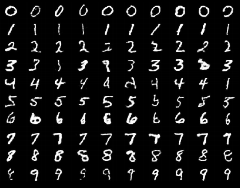
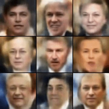
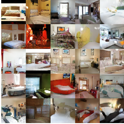
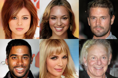
- Deep Belief Network
(Hinton et al. 2006) - Variational AutoEncoder
(Kingma & Welling 2014) - Generative Adversarial Network
(Goodfellow et al. 2014) - Wasserstein GAN
(Arjovsky et al. 2017) - Midjourney v5 Guided Diffusion (2023)
A brief survey of Generative Models Families


- Latent Variable Models:
Assume the following form for the model disribution: $$ x = f_\theta(z) \qquad \mbox{with} \qquad z \sim p(z)$$ This is the case of Generative Adversarial Networks, Variational Auto-Encoders, Normalizing Flows. - Auto-Regressive Models:
Assume an autoregressive decomposition of the signal into products of 1D conditional distributions: $$ p_\theta(x) = p_\theta(x_0) p_\theta(x_1 | x_0) \ldots p_\theta(x_n | x_{n-1}, \ldots x_{0}) $$ This is the case of PixelCNN, GPT-3 - Diffusion Models:
Target distribution generated by a reverse noise diffusion process controled by a Stochastic Differential Equation (SDE).
The Variational Auto-Encoder
- We assume a prior distribution $p(z)$ for the latent variable, and a likelihood $p_\theta(x |z)$ defined by a neural network.
Typically $p_\theta(x|z) = \mathcal{N}(x; f_\theta(x), \sigma^2)$ - Training the generative model amounts to finding $\theta_\star$ that
maximizes the marginal likelihood of the model:
$$p_\theta(x) = \int \mathcal{N}(x; f_\theta(z), \sigma^2) \ p(z) \ dz$$
$\Longrightarrow$ This is generally intractable
- In a VAE, efficient training of parameter $\theta$ is made possible by Amortized Variational Inference.
Auto-Encoding Variational Bayes (Kingma & Welling, 2014)
- We introduce a parametric distribution $q_\phi(z | x)$ which aims to model the posterior $p(z | x)$. We want to minimize $\mathbb{D}_{KL}\left( q_\phi(z | x) \parallel p(z | x) \right)$
- Working out the KL divergence between these two distributions leads to: $$\log p_\theta(x) \quad \geq \quad - \mathbb{D}_{KL}\left( q_\phi(z | x) \parallel p(z) \right) \quad + \quad \mathbb{E}_{z \sim q_{\phi}(. | x)} \left[ \log p_\theta(x | z) \right]$$ $\Longrightarrow$ This is the Evidence Lower-Bound, which is differentiable with respect to $\theta$ and $\phi$.
The famous Variational Auto-Encoder
$$\log p_\theta(x) \geq - \underbrace{\mathbb{D}_{KL}\left( q_\phi(z | x) \parallel p(z) \right)}_{\mbox{code regularization}} + \underbrace{\mathbb{E}_{z \sim q_{\phi}(. | x)} \left[ \log p_\theta(x | z) \right]}_{\mbox{reconstruction error}} $$
Normalizing Flows
Still a latent variable model, except the mapping $f_\theta$ is made to be bijective.
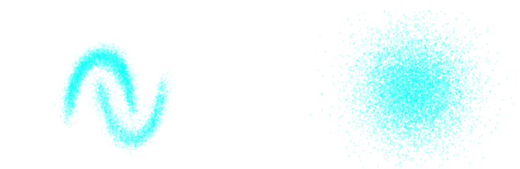
Dinh et al. 2016
Normalizing Flows
- Assumes a bijective mapping between data space $x$ and latent space $z$ with prior $p(z)$: $$ z = f_{\theta} ( x ) \qquad \mbox{and} \qquad x = f^{-1}_{\theta}(z)$$
- Admits an explicit marginal likelihood: $$ \log p_\theta(x) = \log p(z) + \log \left| \frac{\partial f_\theta}{\partial x} \right|(x) $$
$\Longrightarrow$ The challenge is in designing mappings $f_\theta$ that are both:
easy to invert, easy to compute the jacobian of.
One example of NF: RealNVP
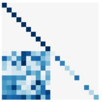
Jacobian of an affine coupling layer
In a standard affine RealNVP, one Flow layer is defined as:
$$ \begin{matrix} y_{1\ldots d} &=& x_{1 \ldots d} \\
y_{d+1\ldots N} &=& x_{d+1 \ldots N} ⊙ \sigma_\theta(x_{1 \ldots d}) + \mu_\theta(x_{1 \ldots d})
\end{matrix} $$
where $\sigma_\theta$ and $\mu_\theta$ are unconstrained neural networks.
We will call this layer an affine coupling.
We will call this layer an affine coupling.
$\Longrightarrow$ This structure has the advantage that the Jacobian of this layer will be lower triangular which makes computing its determinant easy.
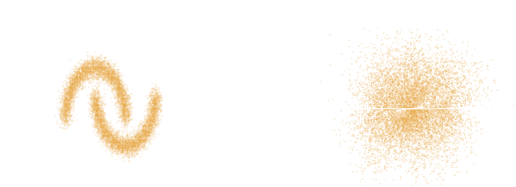
Getting started with Deep Priors: deep denoising example
$$ \boxed{{\color{Orchid} y} = {\color{SkyBlue} x} + n} $$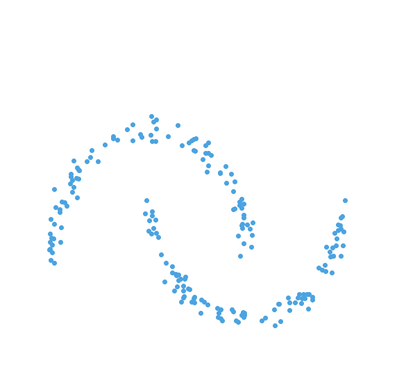
- Let us assume we have access to examples of $ {\color{SkyBlue} x}$ without noise.
- We learn the distribution of noiseless data $\log p_\theta(x)$ from samples using a deep generative model.
- The solution should lie on the realistic data
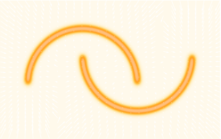
manifold, symbolized by the two-moons distribution.
We want to solve for the Maximum A Posterior solution:
$$\arg \max - \frac{1}{2} \parallel {\color{Orchid} y} - {\color{SkyBlue} x} \parallel_2^2 + \log p_\theta({\color{SkyBlue} x})$$ This can be done by gradient descent as long as one has access to the score function $\frac{\color{orange} d \color{orange}\log \color{orange}p\color{orange}(\color{orange}x\color{orange})}{\color{orange} d \color{orange}x}$.
Back to our motivating example
Hubble Space Telescope
some deep neural network
Simulated Ground-Based Telescope
The issue with generic black box deep learning inference
- No explicit control of noise, PSF, depth.
- Unless covered by the training data, the result becomes unpredictable.
- No guarantees some physical properties are preserved
$\Longrightarrow$ In this case, the flux of the deconvolved object - Robust quantification of uncertainties is extremely difficult.
A Physicist's approach to the deconvolution problem: let's build a model
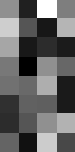
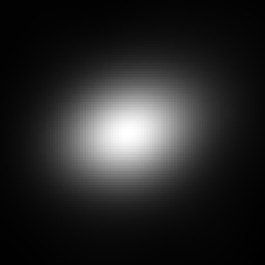
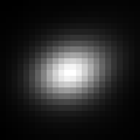
$\longrightarrow$
$g_\theta$
$g_\theta$
$\longrightarrow$
PSF
PSF
$\longrightarrow$
Pixelation
Pixelation
$\longrightarrow$
Noise
Noise
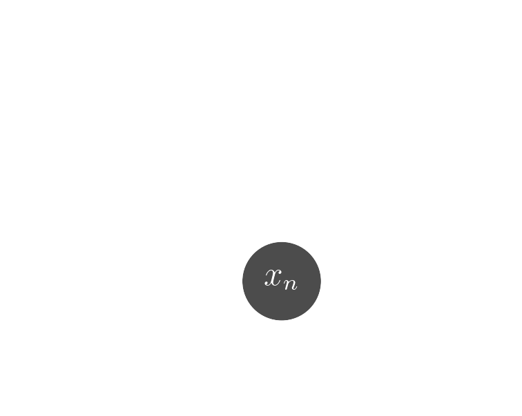
Probabilistic model
$$ x \sim ? $$
$$ x \sim \mathcal{N}(z, \Sigma) \quad z \sim ? $$
latent $z$ is a denoised galaxy image
latent $z$ is a denoised galaxy image
$$ x \sim \mathcal{N}( \mathbf{P} z, \Sigma) \quad z \sim ?$$
latent $z$ is a super-resolved and denoised galaxy image
latent $z$ is a super-resolved and denoised galaxy image
$$ x \sim \mathcal{N}( \mathbf{P} (\Pi \ast z), \Sigma) \quad z \sim ? $$
latent $z$ is a deconvolved, super-resolved, and denoised galaxy image
latent $z$ is a deconvolved, super-resolved, and denoised galaxy image
$$ x \sim \mathcal{N}( \mathbf{P} (\Pi \ast g_\theta(z)), \Sigma) \quad z \sim \mathcal{N}(0, \mathbf{I}) $$
latent $z$ is a Gaussian sample
$\theta$ are parameters of the model
latent $z$ is a Gaussian sample
$\theta$ are parameters of the model
$\Longrightarrow$ Decouples the morphology model from the observing conditions.
How to train your dragon model
- Training the generative amounts to finding $\theta_\star$ that
maximizes the marginal likelihood of the model:
$$p_\theta(x | \Sigma, \Pi) = \int \mathcal{N}( \Pi \ast g_\theta(z), \Sigma) \ p(z) \ dz$$
$\Longrightarrow$ This is generally intractable
- Efficient training of parameter $\theta$ is made possible by Amortized Variational Inference.
Auto-Encoding Variational Bayes (Kingma & Welling, 2014)
- We introduce a parametric distribution $q_\phi(z | x, \Pi, \Sigma)$ which aims to model the posterior $p_{\theta}(z | x, \Pi, \Sigma)$.
- Working out the KL divergence between these two distributions leads to: $$\log p_\theta(x | \Sigma, \Pi) \quad \geq \quad - \mathbb{D}_{KL}\left( q_\phi(z | x, \Sigma, \Pi) \parallel p(z) \right) \quad + \quad \mathbb{E}_{z \sim q_{\phi}(. | x, \Sigma, \Pi)} \left[ \log p_\theta(x | z, \Sigma, \Pi) \right]$$ $\Longrightarrow$ This is the Evidence Lower-Bound, which is differentiable with respect to $\theta$ and $\phi$.
Bayesian Inference a.k.a. Uncertainty Quantification
The Bayesian view of the problem:
$$ p(z | x ) \propto p_\theta(x | z, \Sigma, \mathbf{\Pi}) p(z)$$
where:
- $p( z | x )$ is the posterior
- $p( x | z )$ is the data likelihood, contains the physics
- $p( z )$ is the prior
Data
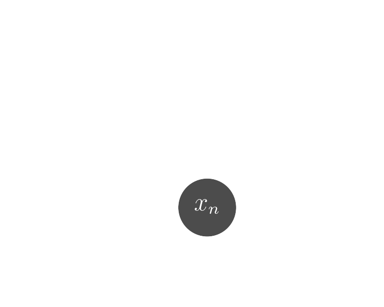
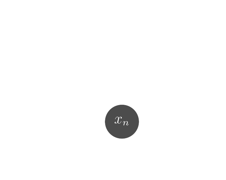
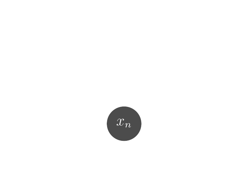
$x_n$
$x_n$
Truth
$x_0$
$x_0$
Posterior samples
$g_\theta(z)$
$g_\theta(z)$
$\mathbf{P} (\Pi \ast g_\theta(z))$
Median
Data residuals
$x_n - \mathbf{P} (\Pi \ast g_\theta(z))$
$x_n - \mathbf{P} (\Pi \ast g_\theta(z))$
Standard Deviation
$\Longrightarrow$ Uncertainties are fully captured by the posterior.
Now you try it!
We will be using this notebook: https://tinyurl.com/inverse-problemYour goal: Solve an image deconvolution problem using a deep generative model as a prior.
Raise your hand when you reach the Maximum Likelihood Solution i.e. end of Step III.
How to solve the posterior inference problem by Variational Inference?
- The core idea of Variational Inference is to assume a model distribution $q_\phi$ and we fit it to the unknown posterior.
- How do we fit a distribution to another distribution? We minize the KL divergence $$ \mathbb{D}_{KL}\left( q_\phi(z) \parallel p(z | x) \right) = \mathbb{E}_{z \sim q_{\phi}} \left[ \log \frac{q_\phi(z)}{p(z | x)} \right] $$$$ = \mathbb{E}_{z \sim q_{\phi}} \left[ \log q(z) \right] - \mathbb{E}_{z \sim q_{\phi}} \left[ \log p(z | x) \right] $$$$ = \mathbb{E}_{z \sim q_{\phi}} \left[ \log q(z) \right] - \mathbb{E}_{z \sim q_{\phi}} \left[ \log p(x | z) + \log p(z) - \log p(x)\right] $$$$ = \underbrace{\mathbb{D}_{KL}\left( q_\phi(z) \parallel p(z) \right) - \mathbb{E}_{z \sim q_{\phi}} \left[ \log p(x | z) \right]}_{\mbox{Evidence Lower Bound}} + \log p(x) $$
- Finally, we need a flexible enough model distribution, why not a Normalizing Flow :-) ?
Modern and Scalable Techniques using Diffusion Models
First realization: The score is all you need!
- Whether you are looking for the MAP or sampling with HMC or MALA, you
only need access to the score of the posterior:
$$\frac{\color{orange} d \color{orange}\log \color{orange}p\color{orange}(\color{orange}x \color{orange}|\color{orange} y\color{orange})}{\color{orange}
d
\color{orange}x}$$
- Gradient descent: $x_{t+1} = x_t + \tau \nabla_x \log p(x_t | y) $
- Langevin algorithm: $x_{t+1} = x_t + \tau \nabla_x \log p(x_t | y) + \sqrt{2\tau} n_t$
- The score of the full posterior is simply: $$\nabla_x \log p(x |y) = \underbrace{\nabla_x \log p(y |x)}_{\mbox{known explicitly}} \quad + \quad \underbrace{\nabla_x \log p(x)}_{\mbox{known implicitly}}$$ $\Longrightarrow$ "all" we have to do is model/learn the score of the prior.
Neural Score Estimation by Denoising Score Matching (Vincent 2011)
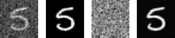
- Denoising Score Matching: An optimal Gaussian denoiser learns the score of a given distribution.
- If $x \sim \mathbb{P}$ is corrupted by additional Gaussian noise $u \in \mathcal{N}(0, \sigma^2)$ to yield $$x^\prime = x + u$$
- Let's consider a denoiser $r_\theta$ trained under an $\ell_2$ loss: $$\mathcal{L}=\parallel x - r_\theta(x^\prime, \sigma) \parallel_2^2$$
- The optimal denoiser $r_{\theta^\star}$ verifies: $$\boxed{\boldsymbol{r}_{\theta^\star}(\boldsymbol{x}', \sigma) = \boldsymbol{x}' + \sigma^2 \nabla_{\boldsymbol{x}} \log p_{\sigma^2}(\boldsymbol{x}')}$$
$\boldsymbol{x}'$
$\boldsymbol{x}$
$\boldsymbol{x}'- \boldsymbol{r}^\star(\boldsymbol{x}', \sigma)$
$\boldsymbol{r}^\star(\boldsymbol{x}', \sigma)$
Second Realization: Annealing is fantastic!
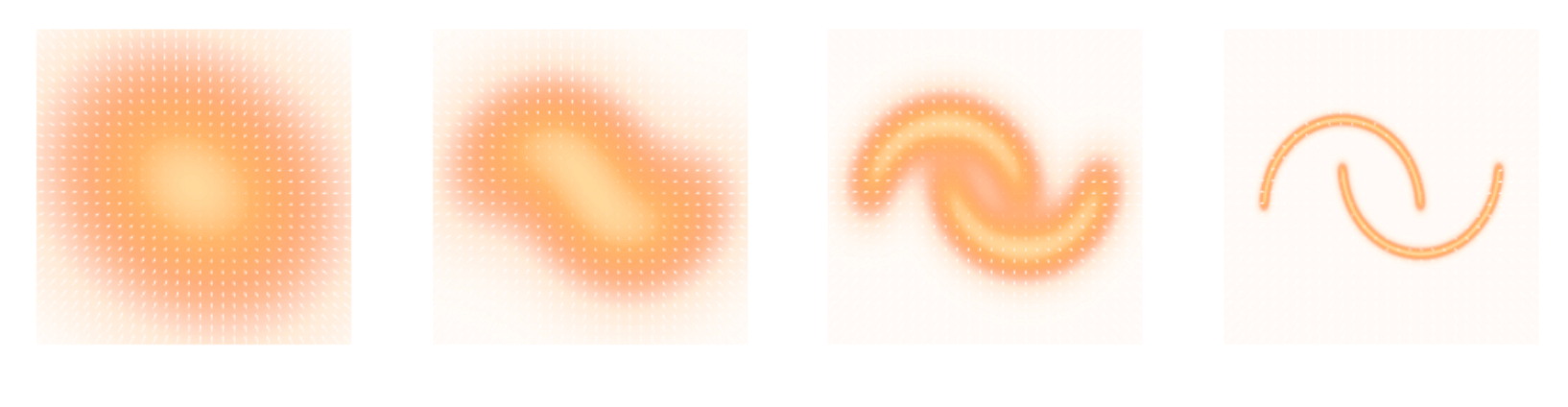
- Even with knowledge of the score, sampling in high number of dimensions is difficult!
- Convolving a target distribution $p$ with a noise kernel, makes $p_\sigma(x) = \int \mathcal{N}(x; x^\prime, \sigma^2) (x^\prime) d x^{\prime}$ it much better behaved
$$\sigma_1 > \sigma_2 > \sigma_3 > \sigma_4 $$
![]()
- Hints to running many MCMC chains in parallel, progressively annealing the $\sigma$ to 0, keep last point in the chain as independent sample.
Score-Based Generative Modeling Song et al. (2021)
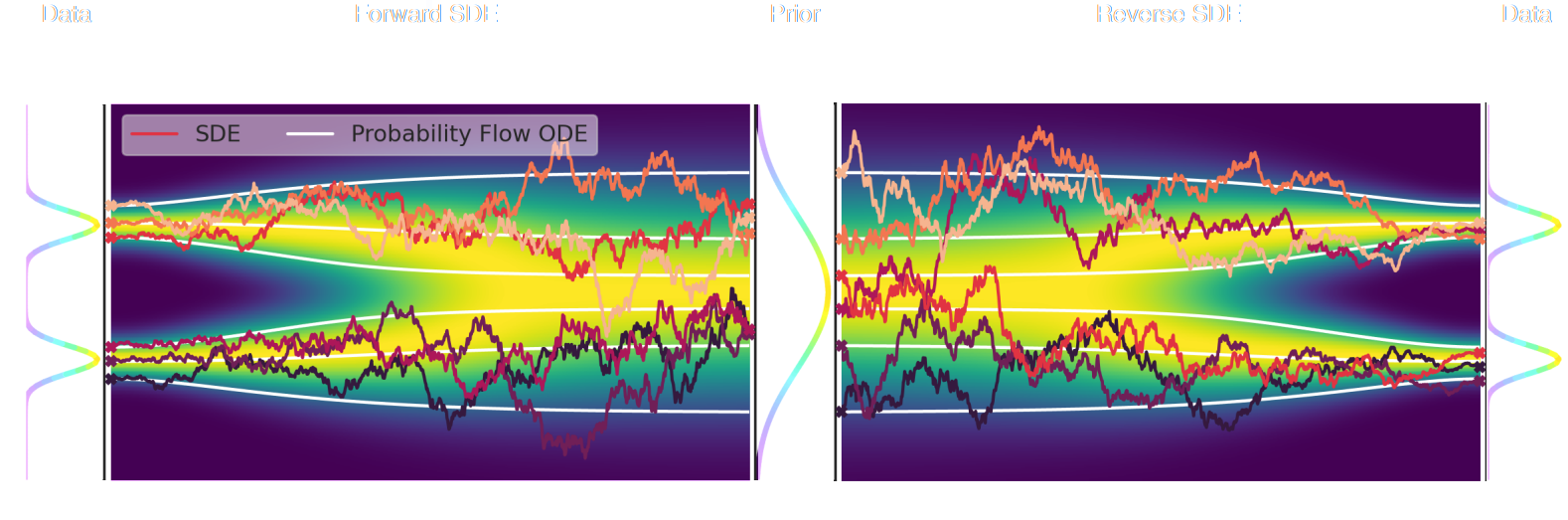
- The SDE defines a marginal distribution $p_t(x)$ as the convolution of the target distribution $p(x)$ with a noise kernel $p_{t|s}(\cdot | x_s)$: $$p_t(x) = \int p(x_s) p_{t|s}(x | x_s) d x_s$$
- For a given forward SDE that evolves $p(x)$ to $p_T(x)$, there exists a reverse SDE that evolves $p_T(x)$ back into $p(x)$. It involves having access to the marginal score $\nabla_x \log_t p(x)$.
But... We don't actually know the marginal posterior score!
- We know the following quantities:
- Annealed likelihood (analytically): $p_\sigma(y | x) = \mathcal{N}(y; \mathbf{A} x, \mathbf{\Sigma} + \sigma^2 \mathbf{I})$
- Annealed prior score (by score matching): $\nabla_x \log p_\sigma(x)$
- But, unfortunately: $\boxed{p_\sigma(x|y) \neq p_\sigma(y|x) \ p_\sigma(x)}$ $\Longrightarrow$ We don't know the marginal posterior score!
- We cannot use the reverse SDE/ODE of diffusion models to sample from the posterior. $$\mathrm{d} x = [f(x, t) - g^2(t) \underbrace{\nabla_x \log p_t(x|y)}_{\mbox{unknown}} ] \mathrm{d}t + g(t) \mathrm{d} w$$
Proposed sampling strategy (Remy et al. 2020)
- Even if not equivalent to the marginal posterior score, $\nabla_x \log p_{\sigma^2}(y | x) + \nabla_x \log p_{\sigma^2}(x)$ still
has good properties:
- Tends to an isotropic Gaussian distribution for large $\sigma$
- Corresponds to the target posterior for $\sigma=0$
- If we simulate this SDE sufficiently slowly (i.e. timescale of change of $\sigma$ is much larger than the timescale of the SDE) we can expect to sample from the target posterior.
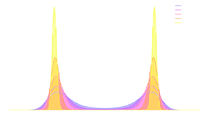
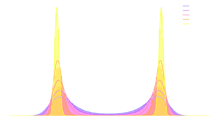
$\Longrightarrow$ In practice, we sample the annealed distribution using an Hamiltonian Monte-Carlo,
with discrete annealing steps.
Approximation methods for the marginal likelihood: DPS (Chung et al. 2023)
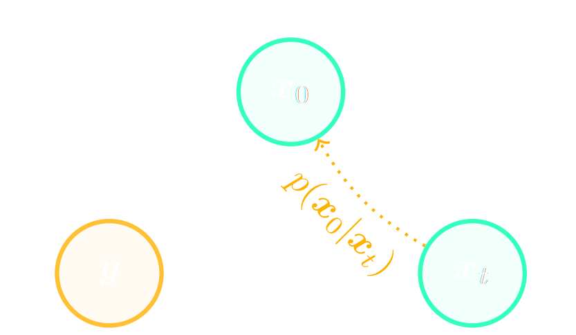
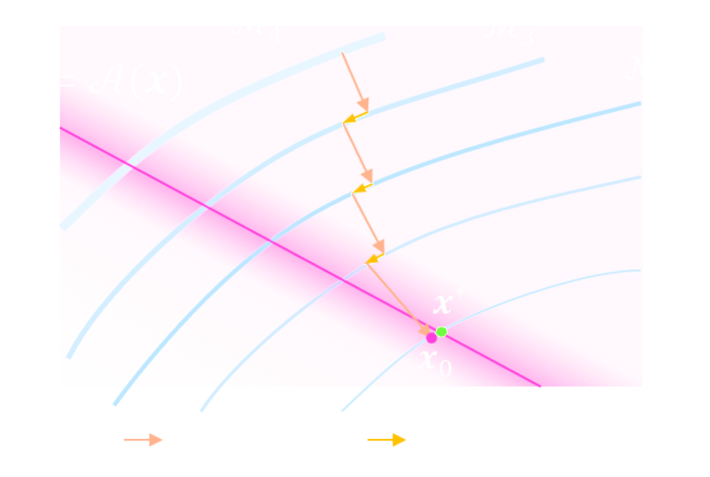
- Let's express the marginal likelihood in terms of x_0:
\begin{align*} p_t(y | x_t) &= \int p(y | x_0) \, p(x_0 | x_t) \, d x_0 \\ &= \mathbb{E}_{x_0 \sim p(x_0 | x_t)}[p(y | x_0)] \end{align*} - The DPS approximation:
$$p(y | x_t) \simeq p(y | \hat{x}_0)$$ with $\hat{x}_0 = \mathbb{E}[x_0 | x_t] = x_t - \sigma_t^2 \nabla_{x_t} \log p_t(x_t)$ - In the case of a Gaussian likelihood and usual linear inverse problem: $$ \nabla_{x_t} \log p_t( y | x_t ) \simeq - \frac{1}{\sigma^2} \nabla_{x_t} \parallel y - \mathbf{A} \hat{x}_0 \parallel_2^2 $$
DPS in practice
Better methods: e.g. Moment Matching Posterior Sampling Rozet et al. 2024
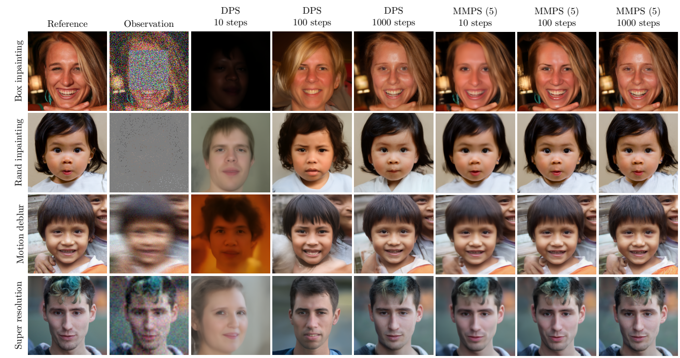 \[
p_t(y \mid x_t) = \int p(y \mid x_0)\, q(x_0 \mid x_t) \, \mathrm{d}x_0
= \mathcal{N}\left(y \mid A\mathbb{E}[x_0 \mid x_t],\, \Sigma_y + A\mathrm{V}[x_0 \mid x_t]A^\top \right)
\]
Advertisement!

Francois Rozet @ University of Liege
from azula.denoise import PreconditionedDenoiser
from azula.noise import VPSchedule
from azula.sample import DDPMSampler

# Choose the variance preserving (VP) noise schedule
schedule = VPSchedule()

# Initialize a denoiser
denoiser = PreconditionedDenoiser(
	backbone=CustomNN(in_features=5, out_features=5),
	schedule=schedule,
)

# Generate 64 points in 1000 steps
sampler = DDPMSampler(denoiser.eval(), steps=1000)

x1 = sampler.init((64, 5))
x0 = sampler(x1)
https://github.com/probabilists/azula
Example of Scientific Application
Let's set the stage: Gravitational lensing
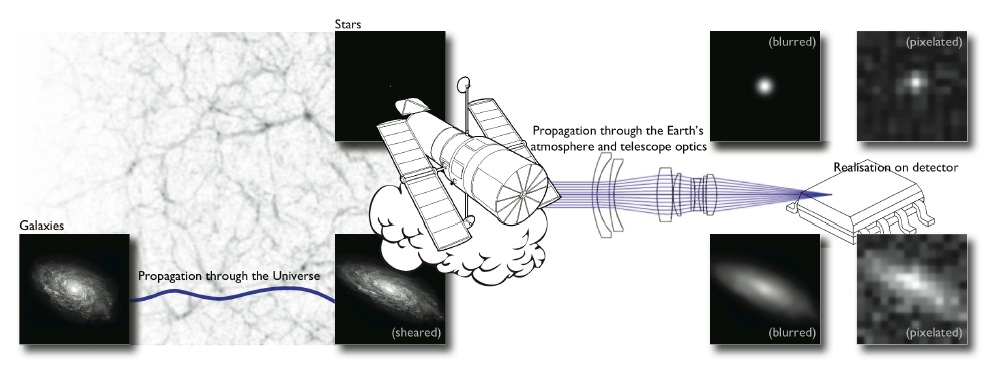
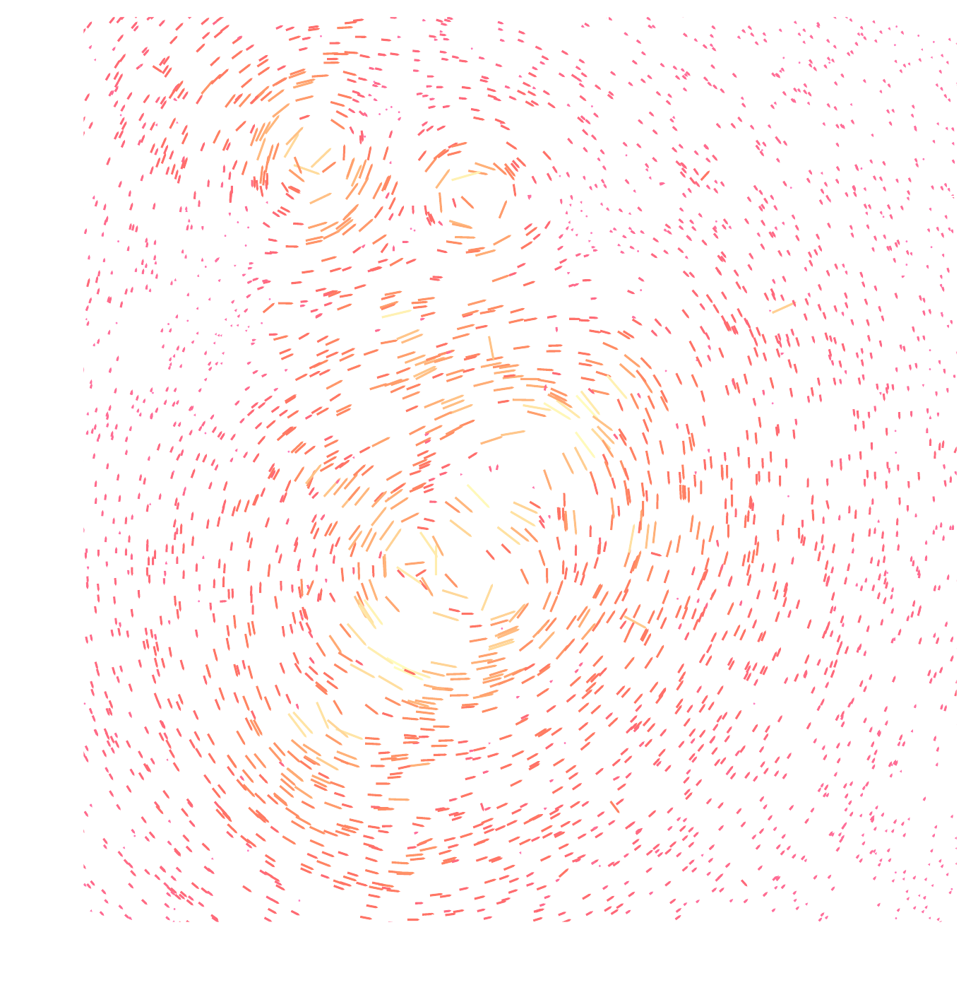
Galaxy shapes as estimators for gravitational shear
$$ e = \gamma + e_i \qquad \mbox{ with } \qquad e_i \sim \mathcal{N}(0, I)$$
- We are trying the measure the ellipticity $e$ of galaxies as an estimator for the gravitational shear $\gamma$
Gravitational Lensing as an Inverse Problem
Shear $\gamma$
![]()
Convergence $\kappa$
![]()
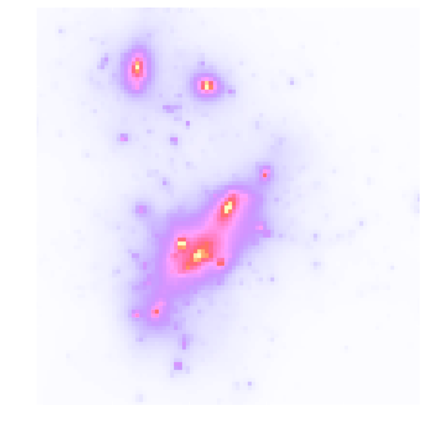
$$\gamma_1 = \frac{1}{2} (\partial_1^2 - \partial_2^2) \ \Psi \quad;\quad \gamma_2 = \partial_1 \partial_2 \ \Psi \quad;\quad \kappa = \frac{1}{2} (\partial_1^2 + \partial_2^2) \ \Psi$$
$$\boxed{\gamma = \mathbf{P} \kappa}$$
Writing down the convergence map log posterior
$$ \log p( \kappa | e) = \underbrace{\log p(e | \kappa)}_{\simeq -\frac{1}{2} \parallel e - P \kappa \parallel_\Sigma^2} + \log p(\kappa) +cst $$- The likelihood term is known analytically, given to us by the physics of gravitational lensing.
- There is no close form expression for the prior on dark matter maps $\kappa$.
However:- We do have access to samples of full implicit prior through simulations: $X = \{x_0, x_1, \ldots, x_n \}$ with $x_i \sim \mathbb{P}$
![]()
- We do have access to samples of full implicit prior through simulations: $X = \{x_0, x_1, \ldots, x_n \}$ with $x_i \sim \mathbb{P}$
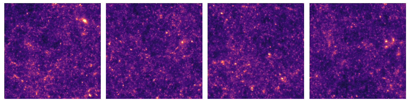
$\Longrightarrow$ Our strategy: Learn the prior from simulation,
and then sample the full posterior.
Example of one chain during Annealed Posterior Sampling
Validating Posterior Sampling under a Gaussian prior
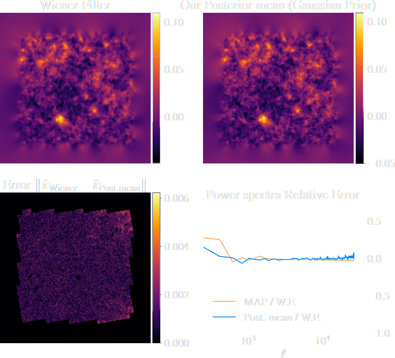
Illustration on $\kappa$-TNG simulations
Remy, Lanusse, et al. (2022) 
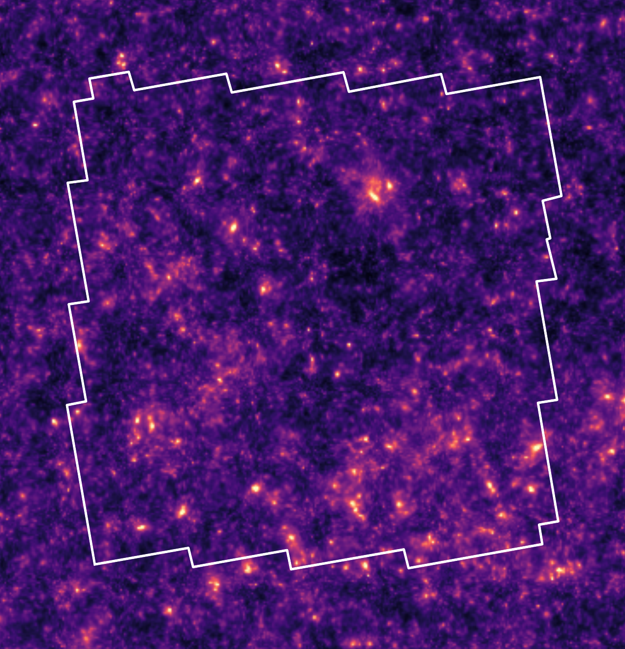
True convergence map
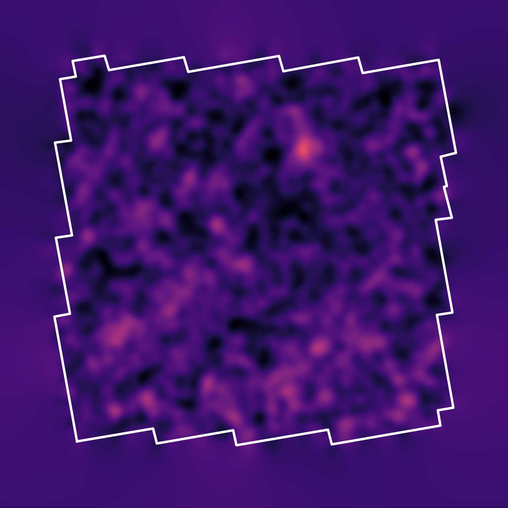
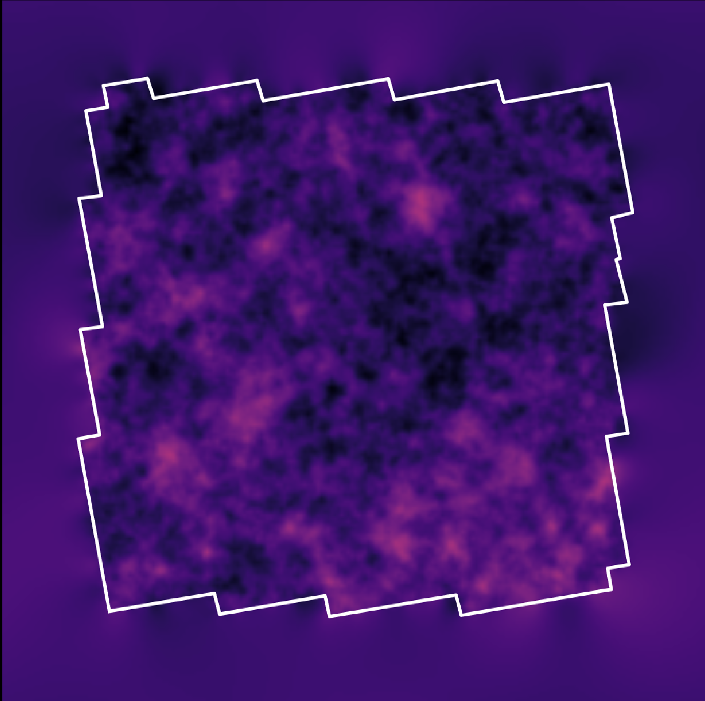
Traditional Kaiser-Squires
Wiener Filter
Posterior Mean (ours)
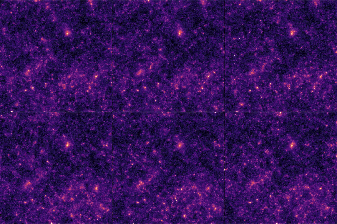
Posterior samples
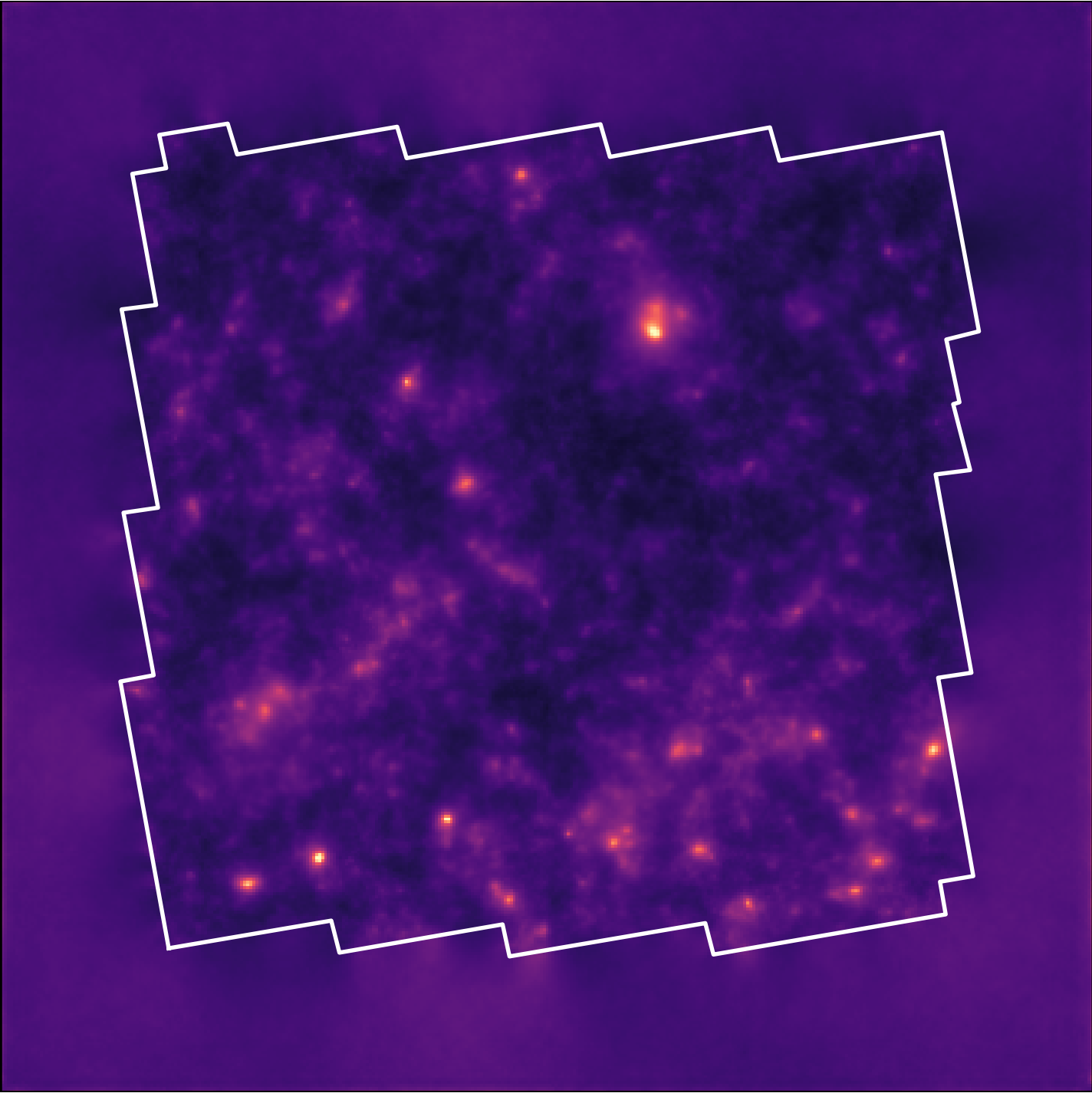
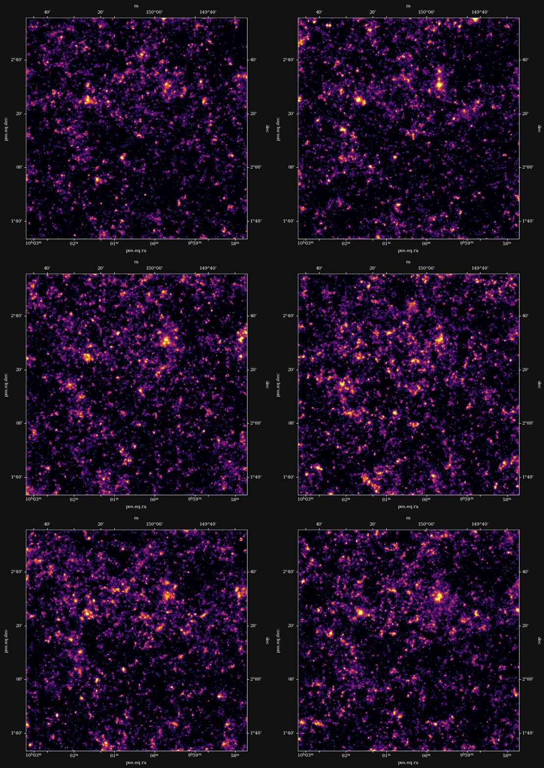
Reconstruction of the HST/ACS COSMOS field
- COSMOS shear data from Schrabback et al. 2010
- Prior learned from $\kappa$-TNG simulation from Osato et al. 2021.
Massey et al. (2007)
![]()
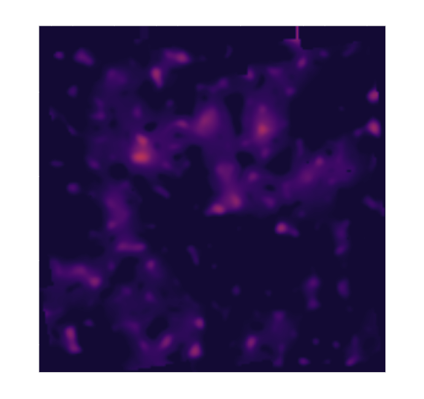
Remy et al. (2022) Posterior mean
![]()
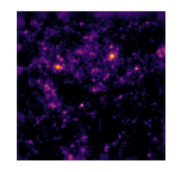
Remy et al. (2022) Posterior samples
![]()
Other examples of Deep Priors
- Hybrid Physical-Deep Learning Model for Astronomical Inverse Problems
F. Lanusse, P. Melchior, F. Moolekamp


$\mathcal{L} = \frac{1}{2} \parallel \mathbf{\Sigma}^{-1/2} (\ Y - P \ast A S \ ) \parallel_2^2 - \sum_{i=1}^K \log p_{\theta}(S_i)$

- Denoising Score-Matching for Uncertainty Quantification in Inverse Problems
Z. Ramzi, B. Remy, F. Lanusse, P. Ciuciu, J.L. Starck