Simulation-Based Bayesian Inference for Cosmology
Dark Universe Summer School, Les Houches, July 2025
François Lanusse


slides at eiffl.github.io/talks/LesHouches2025
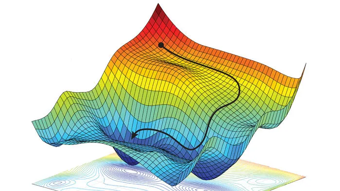
The limits of traditional cosmological inference
HSC cosmic shear power spectrum
HSC Y1 constraints on $(S_8, \Omega_m)$
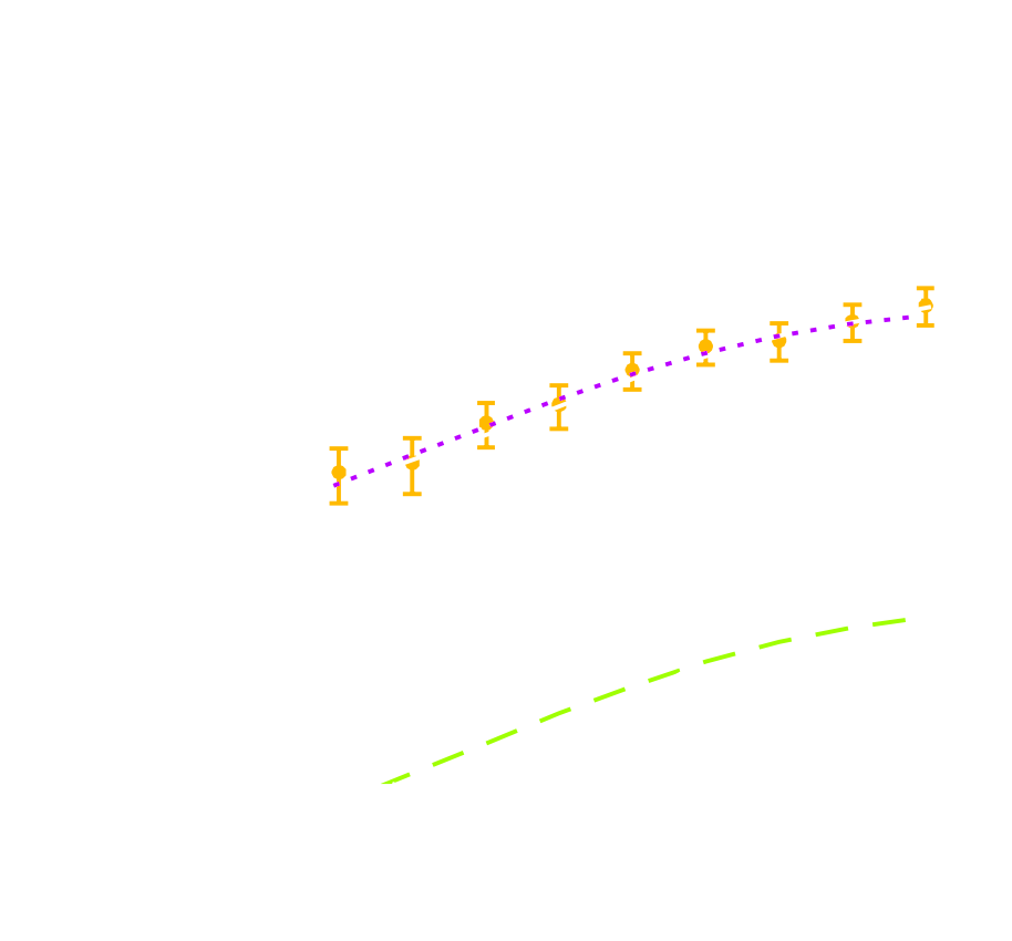
(Hikage et al. 2018)
- Measure the ellipticity $\epsilon = \epsilon_i + \gamma$ of all galaxies
$\Longrightarrow$ Noisy tracer of the weak lensing shear $\gamma$ - Compute summary statistics based on 2pt functions,
e.g. the power spectrum - Run an MCMC to recover a posterior on model parameters, using an analytic likelihood $$ p(\theta | x ) \propto \underbrace{p(x | \theta)}_{\mathrm{likelihood}} \ \underbrace{p(\theta)}_{\mathrm{prior}}$$
Main limitation: the need for an explicit likelihood
We can only compute from theory the likelihood for simple summary statistics and on large scales
$\Longrightarrow$ We are dismissing a significant fraction of the information!
Full-Field Bayesian Inference
- Instead of trying to analytically evaluate the likelihood of
sub-optimal summary statistics, let us build a forward model of the full observables.
$\Longrightarrow$ The simulator becomes the physical model.
Benefits of a forward modeling approach
- Fully exploits the information content of the data (aka "full field inference").
- Easy to incorporate systematic effects.
- Easy to combine multiple cosmological probes by joint simulations.
How can we perform Bayesian inference if all we have access to is a simulator?
Learning objectives for this lecture
- Differences and relative benefits between Full-Field Inference, SBI, traditional MCMC, etc...
- Basics of Neural Networks for Density Estimation.
- How Neural Density Estimation enables SBI.
- Practical considerations around deploying SBI for cosmological analyses.
There is More than One Way to Perform Bayesian Inference
Back to the fundamentals
Bayes' theorem
$$\overbrace{p(\theta|d, \mathcal{M})}^{\text{posterior}} = \frac{ \overbrace{p(d|\theta, \mathcal{M})}^{\text{likelihood}} \ \overbrace{p(\theta|\mathcal{M})}^{\text{prior}}}{\underbrace{p(d|\mathcal{M})}_{\text{evidence}}}$$
- The prior is our belief about the model parameters before observing the data.
- The likelihood is the probability distribution of data given particular model parameters $\theta$.
- The posterior is the probability distribution of model parameters given particular data $d$.
$\Longrightarrow$ Classically, we need to be able to evaluate the log posterior $p(\theta|d, \mathcal{M}) \propto \log p(d|\theta, \mathcal{M}) + \log p(\theta|\mathcal{M})$.
Classical Bayesian inference relies on tractable posterior evaluation
Where do likelihoods come from?
Jeffrey, et al. (2021) 
How can I write the likelihood $p(d | \theta)$?
Note: let's ignore masks here for simplicity
- I can represent my map in harmonic space as: $$\kappa(\hat{n}) = \sum_{\ell m} \kappa_{\ell m} Y_{\ell m} (\hat{n})$$
- I can compute the covariance of $\kappa_{\ell m}$ from theory: $$\langle \kappa_{\ell m} \kappa_{\ell' m'} \rangle = C_\ell (\theta) \delta_{\ell \ell'} \delta_{m m'}$$
- If I estimate my angular power spectrum from data with: $$\hat{C}_\ell = \frac{1}{2\ell+1} \sum_{m=-\ell}^{\ell} |\kappa_{\ell m}|^2$$ then by the Central Limit Theorem, for $\ell > 50$: $$ p(\hat{C}_\ell | \theta) \approx \mathcal{N}\left(\hat{C}_\ell ; C_\ell(\theta), \frac{2C_\ell^2(\theta)}{2\ell+1}\right)$$
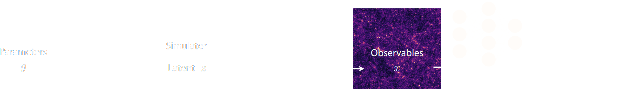
Inference with a Simulation Model
The Challenge of Simulation-Based Inference
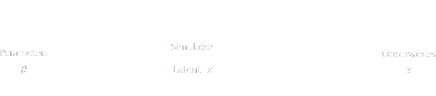
$$ p(x|\theta) = \int p(x, z | \theta) dz = \int p(x | z, \theta) p(z | \theta) dz $$
Where $z$ are stochastic latent variables of the simulator.
$\Longrightarrow$ This marginal likelihood is in general intractable!
$\Longrightarrow$ This marginal likelihood is in general intractable!
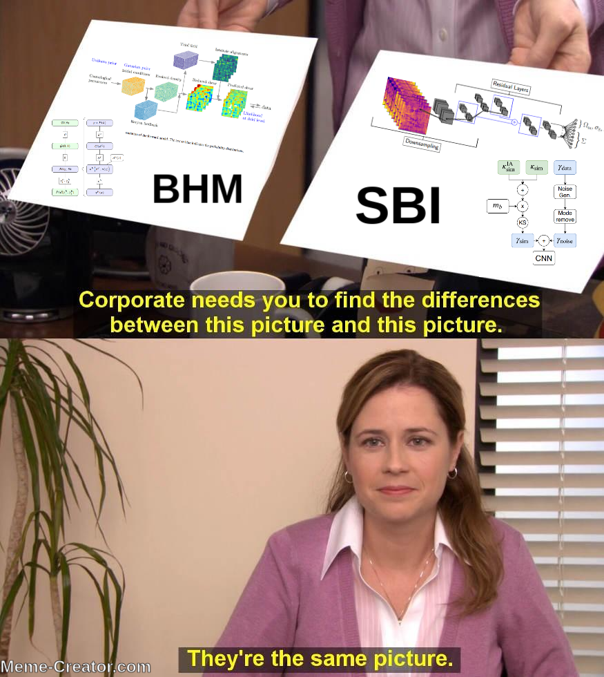
Simulators as Hierarchical Bayesian Models
- If we have access to all latent variables $z$ of the simulator, then the joint log likelihood $p(x | z, \theta)$ is explicit.
- We need to infer the joint posterior $p(\theta, z | x)$ before marginalization to
yield $p(\theta | x) = \int p(\theta, z | x) dz$.
$\Longrightarrow$ Extremely difficult problem as $z$ is typically very high-dimensional. - Necessitates inference strategies with access to gradients of the likelihood. $$\frac{d \log p(x | z, \theta)}{d \theta} \quad ; \quad \frac{d \log p(x | z, \theta)}{d z} $$ For instance: Maximum A Posterior estimation, Hamiltonian Monte-Carlo, Variational Inference.
$\Longrightarrow$ This is what we will call Explicit Inference, because we can evaluate $p(x | z, \theta)$ explicitly.
Black-box Simulators Define Implicit Distributions
- A black-box simulator defines $p(x | \theta)$ as an implicit distribution, you can sample from it but you cannot evaluate it.
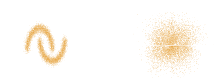
- Key Idea: Use a parametric distribution model $\mathbb{P}_\phi$ to approximate the implicit distribution $\mathbb{P}$.

True $\mathbb{P}$

Samples $x_i \sim \mathbb{P}$

Model $\mathbb{P}_\varphi$
- Once trained, you can typically sample from $\mathbb{P}_\phi$ and/or evaluate the likelihood $p_\phi(x | \theta)$.
How to perform inference over forward simulation models?
- Implicit Inference: Treat the simulator as a black-box with only the ability to sample from the joint distribution
$$(x, \theta) \sim p(x, \theta)$$
a.k.a.
- Simulation-Based Inference (SBI)
- Likelihood-free inference (LFI)
- Approximate Bayesian Computation (ABC)
- Explicit Inference: Treat the simulator as a probabilistic model and perform inference over the joint posterior
$$p(\theta, z | x) \propto p(x | z, \theta) p(z, \theta) p(\theta) $$
a.k.a.
- Bayesian Hierarchical Modeling (BHM)
$\Longrightarrow$ For a given simulation model, both methods should converge to the same posterior!
Neural Density Estimation
The key to manipulating Implicit Distributions
What is a neural network?
Simplest architecture: Multilayer Perceptron (MLP)
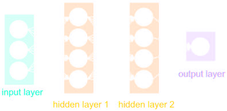
- Series of Dense a.k.a Fully connected layers:
$$ h = \sigma(W x + b)$$
where:
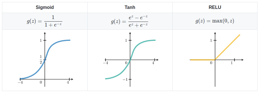
- $\sigma$ is the activation function (e.g. ReLU, Sigmoid, etc.)
- $W$ is a multiplicative weight matrix
- $b$ is an additive bias parameter
- This defines a parametric non-linear function $f_\theta(x)$
- MLPs are universal function approximators
Nota bene: only asymptotically true!
How do you use it to approximate functions?
- Assume a loss function that should be small for good approximations on a training set of data points $(x_i, y_i)$ $$ \mathcal{L} = \sum_{i} ( y_i - f_\theta(x_i))^2 $$
- Optimize the parameters $\theta$ to minimize the loss function by gradient descent $$ \theta_{t+1} = \theta_t - \eta \nabla_\theta \mathcal{L} $$
The task at hand: Density Estimation
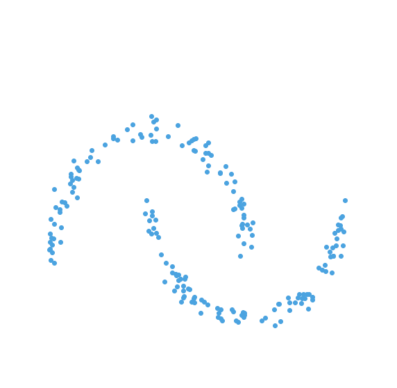
- The goal of density estimation is to estimate an implicit distribution $\mathbb{P}$ from which a training set $X = \{x_0, x_1, \ldots, x_n \}$ is drawn.
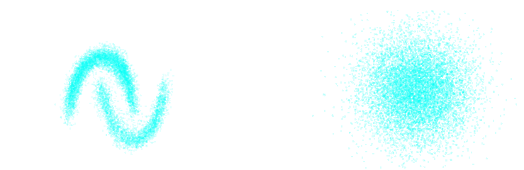
- Usually, this means building a parametric model $\mathbb{P}_\phi$ that tries to be close to $\mathbb{P}$.
True $\mathbb{P}$
Samples $x_i \sim \mathbb{P}$
Model $\mathbb{P}_\phi$
- How do we do this?
 The Kullback-Leibler divergence:
\begin{align}
D_{KL}(p||q_\phi) &= \mathbb{E}_{x \sim p(x)} \left[ \log \frac{p(x)}{q_\phi(x)} \right] \\ \\
&= - \mathbb{E}_{x \sim p(x)} \left[ \log q_\phi(x) \right] + \underbrace{H(p)}_{\text{const}}
\end{align}
The Kullback-Leibler divergence:
\begin{align}
D_{KL}(p||q_\phi) &= \mathbb{E}_{x \sim p(x)} \left[ \log \frac{p(x)}{q_\phi(x)} \right] \\ \\
&= - \mathbb{E}_{x \sim p(x)} \left[ \log q_\phi(x) \right] + \underbrace{H(p)}_{\text{const}}
\end{align}
- Step I: We need a parametric density model $q_\phi(x)$
Simplest possible model, a parametric Gaussian: $$ q_\phi(x) = \mathcal{N}(x ; \mu, \Sigma) $$ with parameters $\phi = \{\mu, \Sigma\}$ - Step II: We need a tool to compare distributions
- Step III: We optimize the parameters $\phi$ to minimize the NLL over a training set $X = \{x_1, x_2, \ldots, x_N\} \sim \mathbb{P}$ : $$ \mathcal{L}(\phi) = - \frac{1}{N} \sum_{i=1}^N \log q_\phi(x_i) $$ $\Longrightarrow$ This will minimize the KL divergence and fit the model to the data.
Your goto NDE in low dimensions (<100): The Normalizing Flows
Dinh et al. 2016
Normalizing Flows
- Assumes a bijective mapping between data space $x$ and latent space $z$ with known $p(z)$: $$ z = f_{\theta} ( x ) \qquad \mbox{and} \qquad x = f^{-1}_{\theta}(z)$$
- Admits an explicit marginal likelihood: $$ \log p_\theta(x) = \log p(z) + \log \left| \frac{\partial f_\theta}{\partial x} \right|(x) $$
$\Longrightarrow$ The challenge is in designing mappings $f_\theta$ that are both:
easy to invert, easy to compute the jacobian of.
One example of NF: RealNVP
Jacobian of an affine coupling layer
In a standard affine RealNVP, one Flow layer is defined as:
$$ \begin{matrix} y_{1\ldots d} &=& x_{1 \ldots d} \\
y_{d+1\ldots N} &=& x_{d+1 \ldots N} ⊙ \sigma_\theta(x_{1 \ldots d}) + \mu_\theta(x_{1 \ldots d})
\end{matrix} $$
where $\sigma_\theta$ and $\mu_\theta$ are unconstrained neural networks.
We will call this layer an affine coupling.
We will call this layer an affine coupling.
$\Longrightarrow$ This structure has the advantage that the Jacobian of this layer will be lower triangular which makes computing its determinant easy.
Your Turn!
You can take a look at this notebook to implement a Normalizing Flow in JAX+Flax+TensorFlow Probability
Implicit Inference
Black-box Simulators Define Implicit Distributions
- A black-box simulator defines $p(x | \theta)$ as an implicit distribution, you can sample from it but you cannot evaluate it.
- This gives us a procedure to sample from the Bayesian joint distribution $p(x, \theta)$: $$(x, \theta) \sim p(x | \theta) \ p(\theta)$$
- Key Idea: Use a parametric distribution model to approximate an implicit distribution.
- Neural Likelihood Estimation: $\mathcal{L} = - \mathbb{E}_{(x,\theta)}\left[ \log p_\phi( x | \theta ) \right] $
- Neural Posterior Estimation: $\mathcal{L} = - \mathbb{E}_{(x,\theta)}\left[ \log p_\phi( \theta | x ) \right] $
- Neural Ratio Estimation: $\mathcal{L} = - \mathbb{E}_{\begin{matrix} (x,\theta)~p(x,\theta) \\ \ \theta^\prime \sim p(\theta) \end{matrix}} \left[ \log r_\phi(x,\theta) + \log(1 - r_\phi(x, \theta^\prime)) \right] $
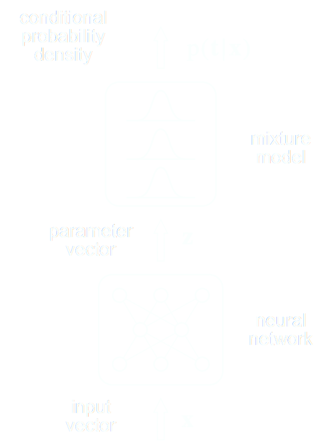
A closer look at Neural Posterior Estimation (NPE)
- Building conditional neural density estimators $q_\phi(\theta | x)$ to approximate the posterior
![]()
Bishop (1994)
- Bounding the KL divergence between true and approximate posterior
$$D_{KL}(p(x | y) ||q_\phi(x | y)) = \mathbb{E}_{x \sim p(x |y)} \left[ \log \frac{p(x | y)}{q_\phi(x | y)} \right] \geq 0 $$$$ \leq \mathbb{E}_{y \sim p(y)} \mathbb{E}_{x \sim p(x |y)} \left[ \log \frac{p(x | y)}{q_\phi(x | y)} \right] $$$$ \leq \boxed{ \mathbb{E}_{(y,x) \sim p(y, x)} \left[ - \log q_\phi(x | y) \right] } + cst $$
$\Longrightarrow$ Minimizing the Negative Log Likelihood (NLL) over the joint distribution $p(x, y)$ leads to minimizing the KL divergence between the model posterior $q_{\phi}(x|y)$ and true posterior $p(x | y)$.
The NPE recipe
- I assume a forward model of the observations: \begin{equation} p( x ) = p(x | \theta) \ p(\theta) \nonumber \end{equation} All I ask is the ability to sample from the model, to obtain $\mathcal{D} = \{x_i, \theta_i \}_{i\in \mathbb{N}}$
- I am going to assume $q_\phi(\theta | x)$ a parametric conditional density
- Optimize the parameters $\phi$ of $q_{\phi}$ according to \begin{equation} \min\limits_{\phi} \sum\limits_{i} - \log q_{\phi}(\theta_i | x_i) \nonumber \end{equation} In the limit of large number of samples and sufficient flexibility \begin{equation} \boxed{q_{\phi^\ast}(\theta | x) \approx p(\theta | x)} \nonumber \end{equation}
$\Longrightarrow$ One can asymptotically recover the posterior by
optimizing a parametric estimator over
the Bayesian joint distribution
the Bayesian joint distribution
$\Longrightarrow$ One can asymptotically recover the posterior by
optimizing a Deep Neural Network over
a simulated training set.
a simulated training set.
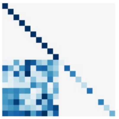
A variety of algorithms
Lueckmann, Boelts, Greenberg, Gonçalves, Macke (2021) 
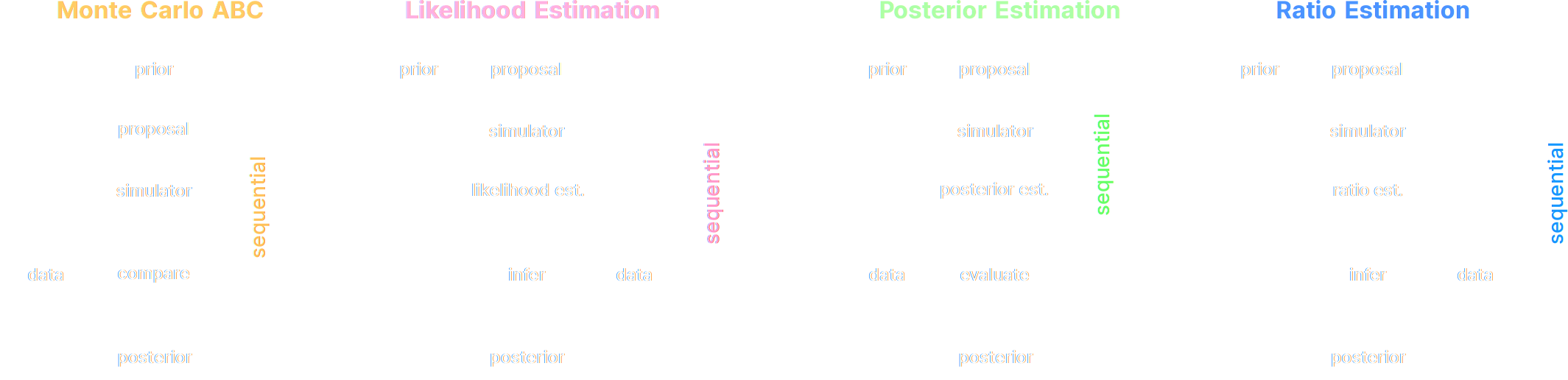
A few important points:
- Amortized inference methods, which estimate $p(\theta | x)$, can greatly speed up posterior estimation once trained.
- Sequential SBI algorithms can actively sample simulations needed to refine the inference.
Checkout this excellent package: https://www.mackelab.org/sbi
A Practical Recipe for Careful Simulation-Based Inference
Estimating conditional densities
in high dimensions is hard...
To be more robust, you can decompose the problem into two tasks:
- Step I - Dimensionality Reduction: Compress your observables $x$ to a low dimensional summary statistic $y$
![]()
- Step II - Conditional Density Estimation: Estimate the posterior $p(\theta | y)$ using SBI from the low dimensional summary statistic $y$.
The Case for Dimensionality Reduction
- In the case of Neural Posterior Estimation
![]()
![]() $p(\theta | x)$$\Longrightarrow$ Dimensionality reduction already happens implicitly in the network.
$p(\theta | x)$$\Longrightarrow$ Dimensionality reduction already happens implicitly in the network. - In the case of Neural Likelihood Estimation
![]() $x \sim p(x|\theta)$
$x \sim p(x|\theta)$
![]() $\theta$$\Longrightarrow$ This is equivalent to learning a perfect emulator for the high-dimensional outputs of your numerical simulator.
$\theta$$\Longrightarrow$ This is equivalent to learning a perfect emulator for the high-dimensional outputs of your numerical simulator.
How can we lower the dimensionality of the problem without degrading our constraining power?
Automated Neural Summarization
- Introduce a parametric function $f_\varphi$ to reduce the dimensionality of the data while preserving information.
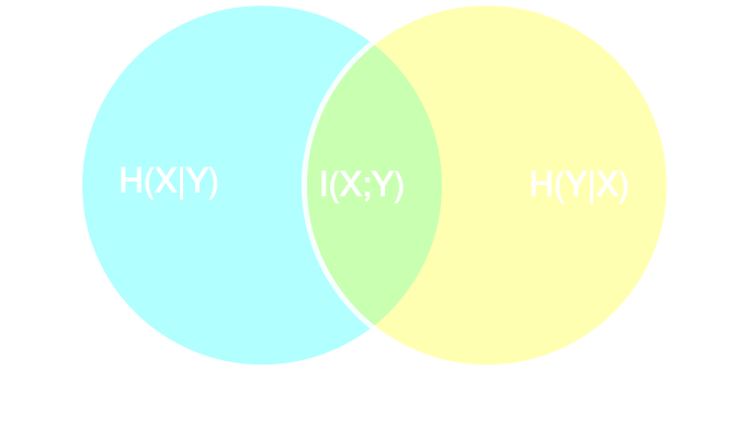
Information point of view
- Summary statistics $y$ is sufficient for $\theta$ if $$ I(Y; \Theta) = I(X; \Theta) \Leftrightarrow p(\theta | x ) = p(\theta | y) $$
- Variational Mutual Information Maximization
$$ \mathcal{L} \ = \ \mathbb{E}_{x, \theta} [ \log q_\phi(\theta | y=f_\varphi(x)) ] \leq I(Y; \Theta) $$
(Barber & Agakov variational lower bound)
Jeffrey, Alsing, Lanusse (2021)

Another Approach: maximizing the Fisher information
 Information Maximization Neural Network (IMNN)
$$\mathcal{L} \ = \ - | \det \mathbf{F} | \ \mbox{with} \ \mathbf{F}_{\alpha, \beta} = tr[ \mu_{\alpha}^t C^{-1} \mu_{\beta} ] $$
Information Maximization Neural Network (IMNN)
$$\mathcal{L} \ = \ - | \det \mathbf{F} | \ \mbox{with} \ \mathbf{F}_{\alpha, \beta} = tr[ \mu_{\alpha}^t C^{-1} \mu_{\beta} ] $$
Charnock, Lavaux, Wandelt (2018) 
Conventional Recipe for Full-Field Implicit Inference...
A two-steps approach to Implicit Inference
- Automatically learn an optimal low-dimensional summary statistic $$y = f_\varphi(x) $$
- Use Neural Density Estimation to either:
- build an estimate $p_\phi$ of the likelihood function $p(y \ | \ \theta)$ (Neural Likelihood Estimation)
- build an estimate $p_\phi$ of the posterior distribution $p(\theta \ | \ y)$ (Neural Posterior Estimation)
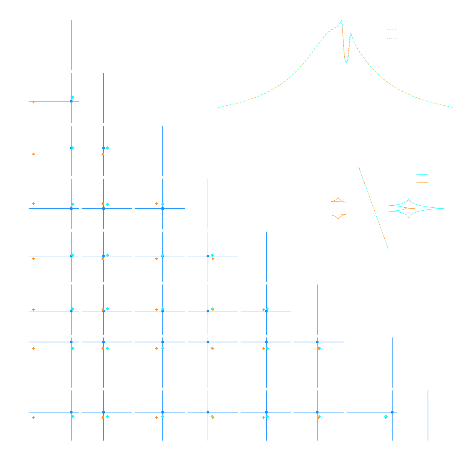
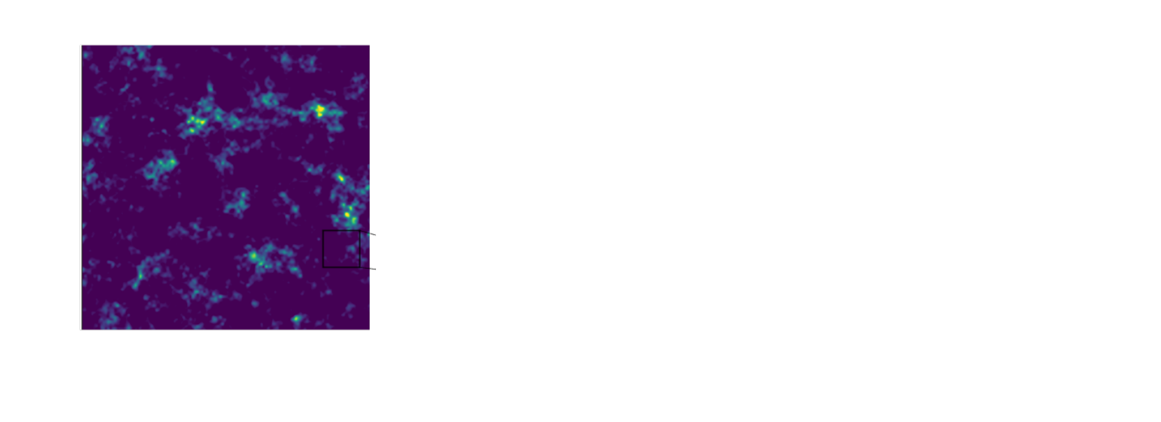
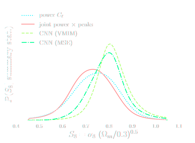
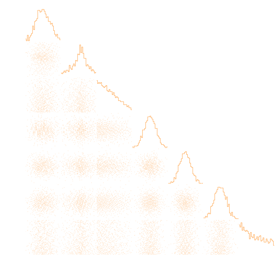
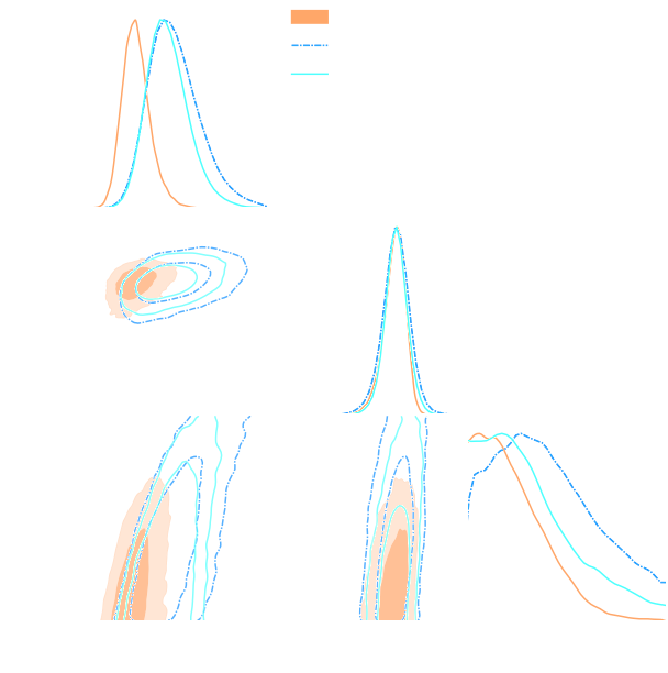
Validation on log-normal lensing simulations

DifferentiableUniverseInitiative/sbi_lens
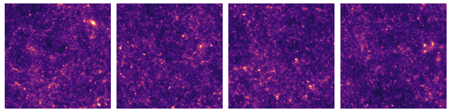
JAX-based log-normal lensing simulation package
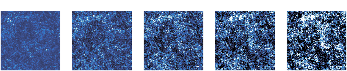
- 10x10 deg$^2$ maps at LSST Y10 quality, conditioning the log-normal shift parameter on $(\Omega_m, \sigma_8, w_0)$
- Infer full-field posterior on cosmology:
- explicitly using an Hamiltonian-Monte Carlo (NUTS) sampler
- implicitly using a learned summary statistics and conditional density estimation.
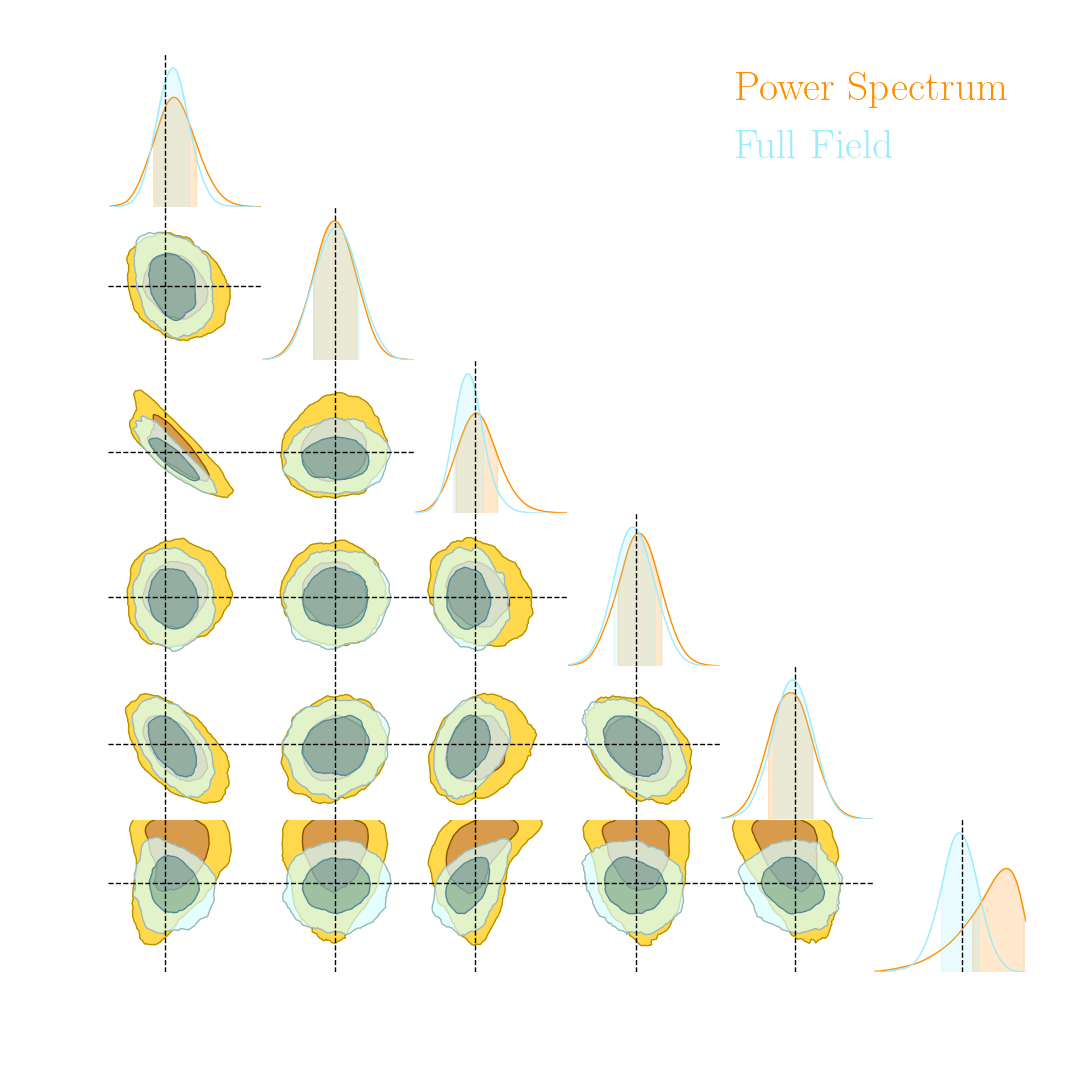
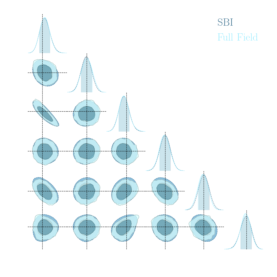
Note: not all compression techniques are equivalent!
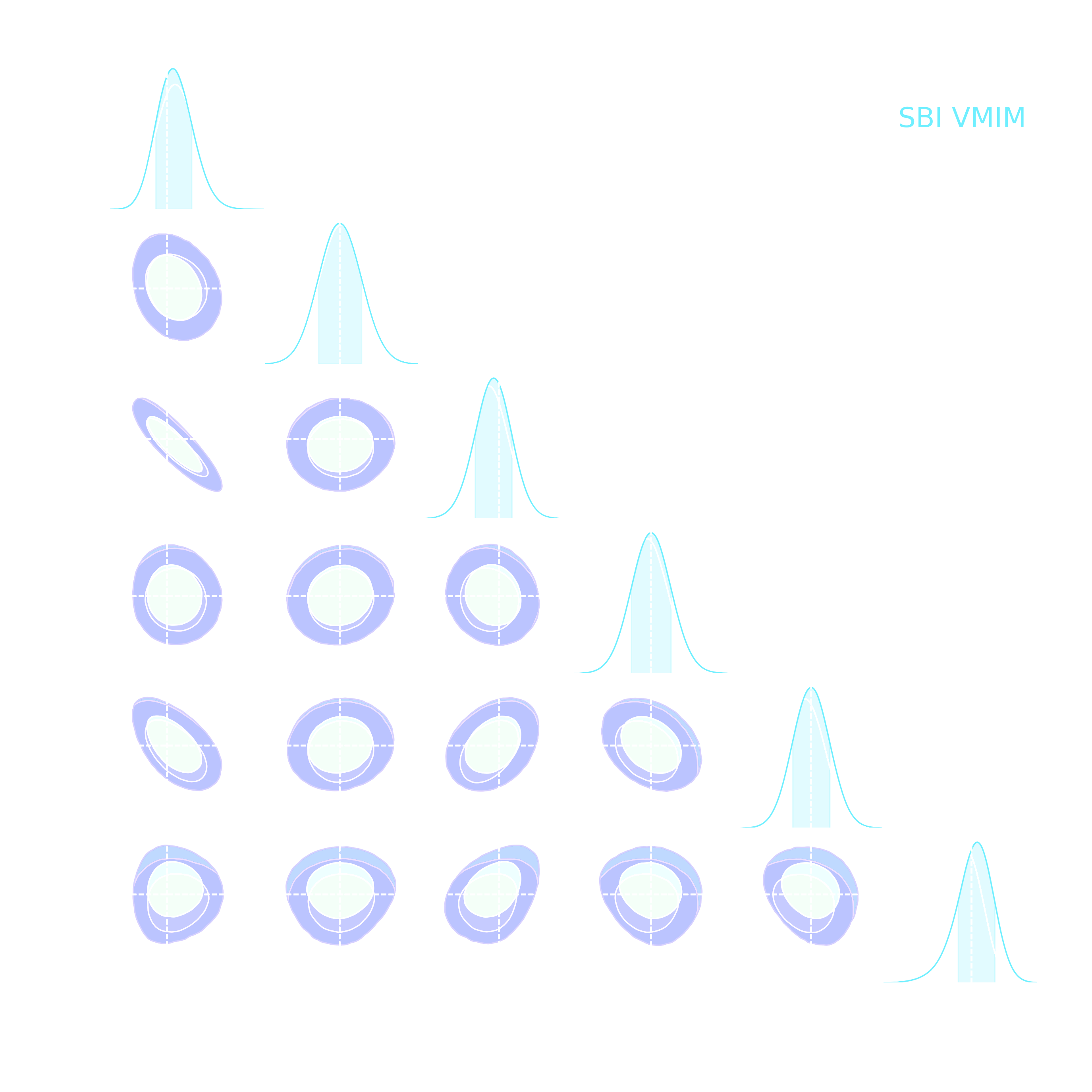
- Comparison to posteriors obtained with same neural compression architecture, but different loss function: $$\mathcal{L}_{MSE} = \mathbb{E}_{(x,\theta)} || f_\varphi(x) - \theta ||_2^2 $$
How can I build efficient and robust SBI analyses?
A neural network will try to answer
the question you ask.
A Simple Strategy to Evaluate Epistemic Errors: Ensembles of NDEs


Verifying Proper Coverage


Applications
Our humble beginnings: Likelihood-Free Parameter Inference with DES SV...
Jeffrey, Alsing, Lanusse (2021) 
Suite of N-body + raytracing simulations: $\mathcal{D}$
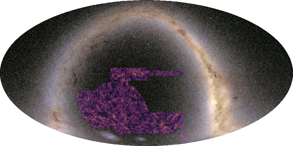
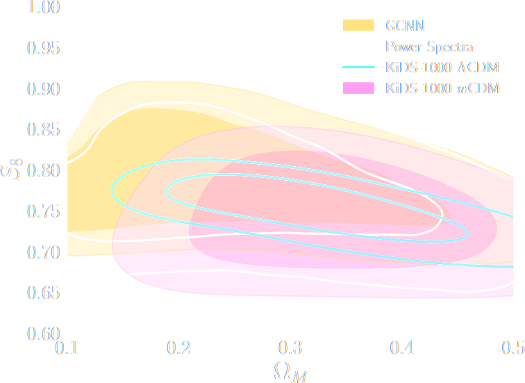
$w$CDM analysis of KiDS-1000 Weak Lensing (Fluri et al. 2022)
Fluri, Kacprzak, Lucchi, Schneider, Refregier, Hofmann (2022)

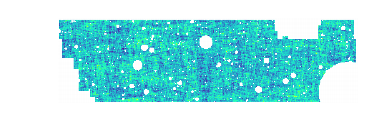
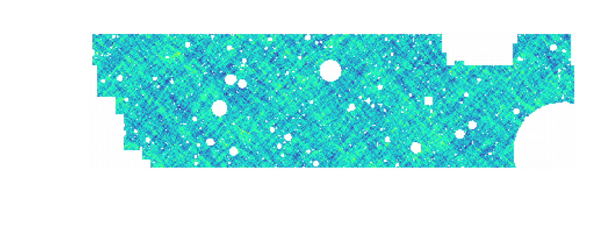
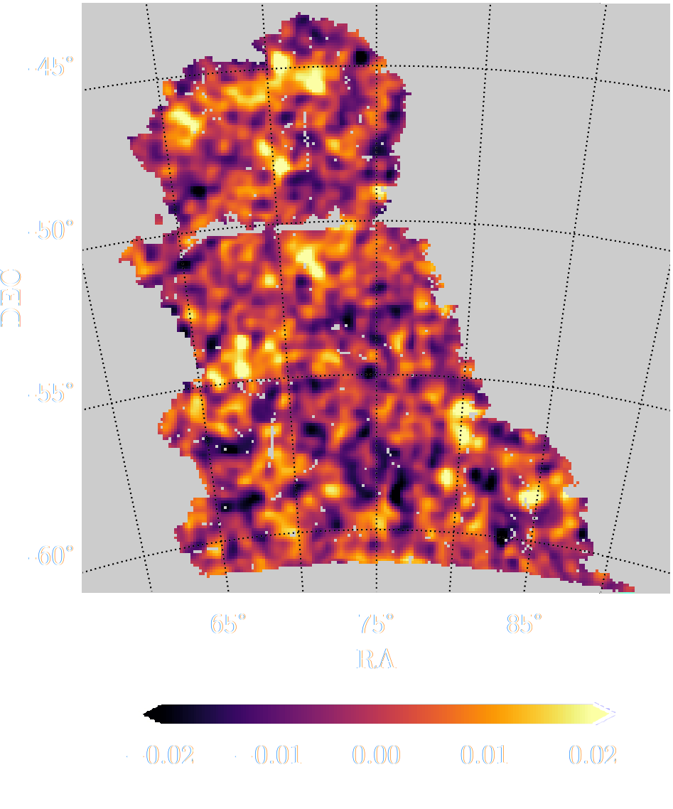
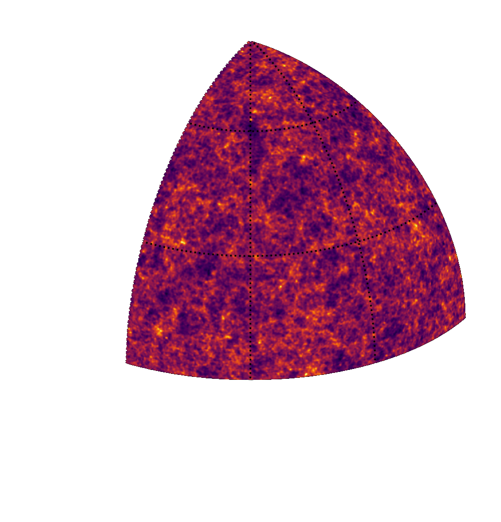
KiDS-1000 footprint and simulated data
![]()
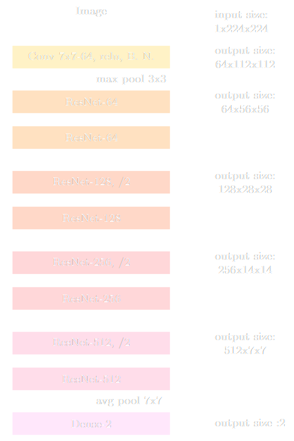
- Neural Compressor: Graph Convolutional Neural Network on the Sphere
Trained by Fisher information maximization.
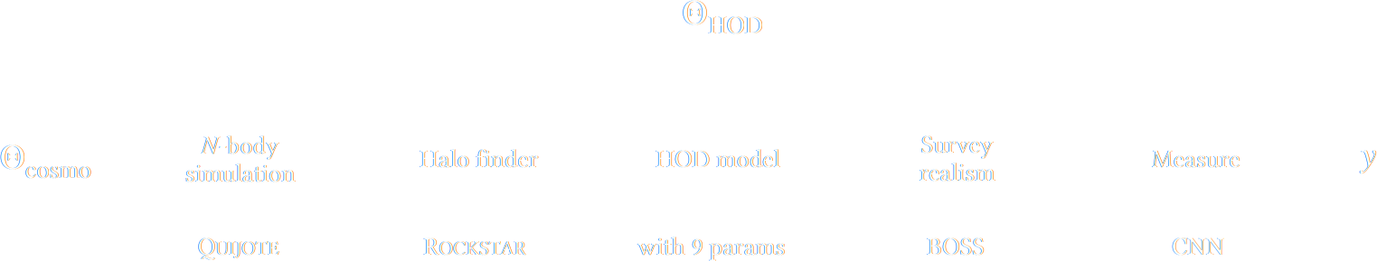
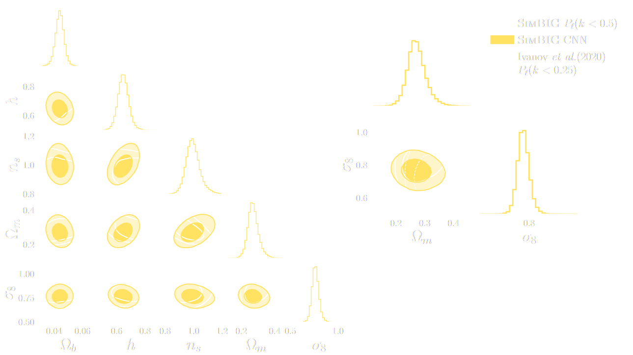
SIMBIG: Field-level SBI of Large Scale Structure (Lemos et al. 2023)
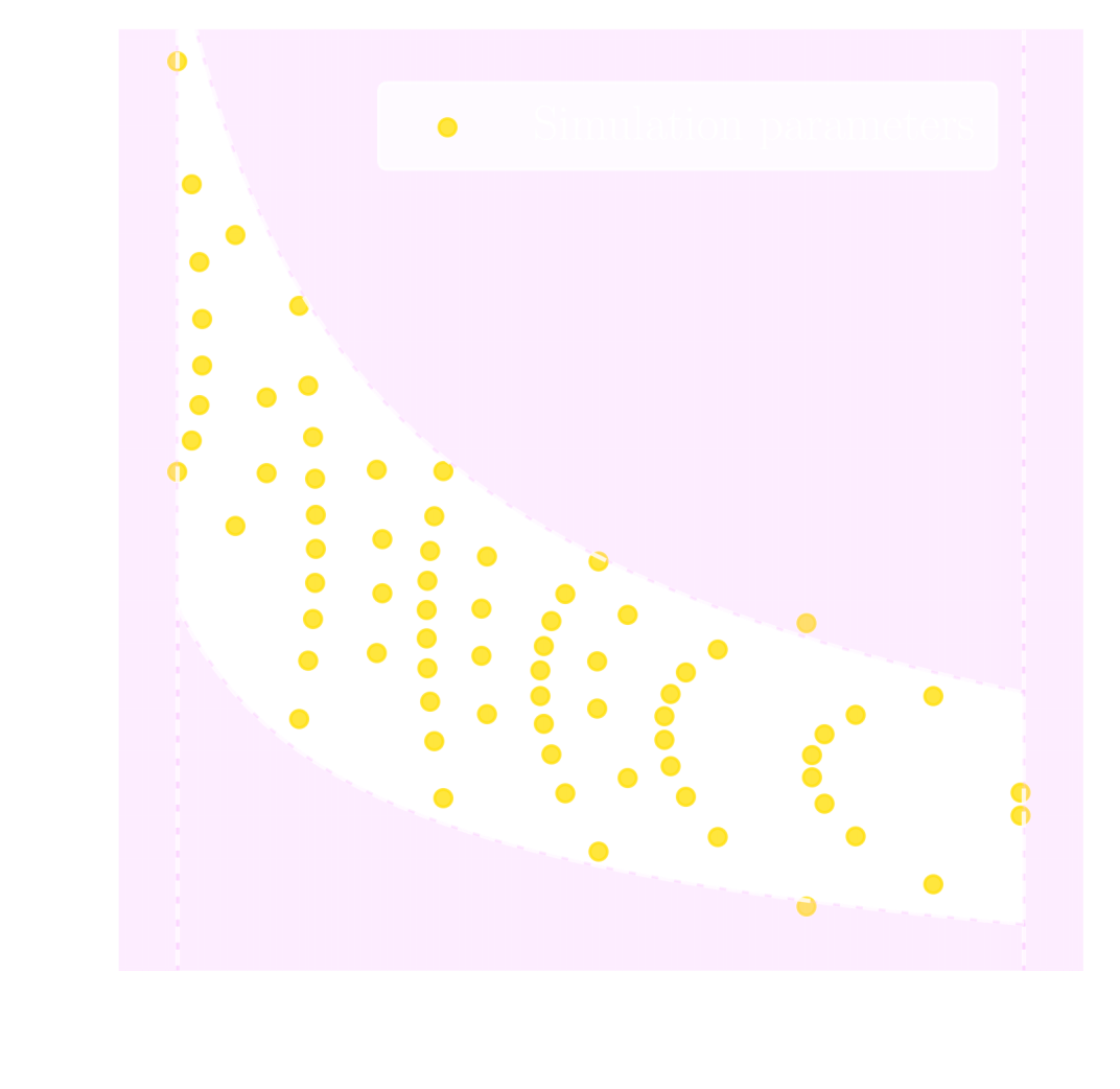
BOSS CMASS galaxy sample: Data vs Simulations
- 20,000 simulated galaxy samples at 2,000 cosmologies
Hahn et al. (2022)

Finally, SBI has reached the mainstream: Official DES year 3 SBI wCDM results
Jeffrey et al. (2024)

Can we just retire all conventional likelihood-based analyses?
Example of unforeseen impact of shortcuts in simulations
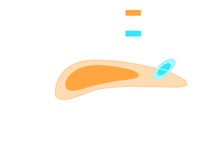
Gatti, Jeffrey, Whiteway et al. (2023)

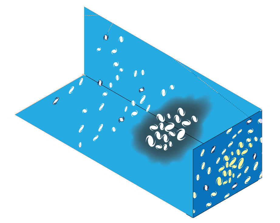
Is it ok to distribute lensing source galaxies randomly in simulations, or should they be clustered?
$\Longrightarrow$ An SBI analysis could be biased by this effect and you would never know it!
How much usable information is there beyond the power spectrum?
Chisari et al. (2018)

Ratio of power spectrum in hydrodynamical simulations vs. N-body simulations
Secco et al. (2021)

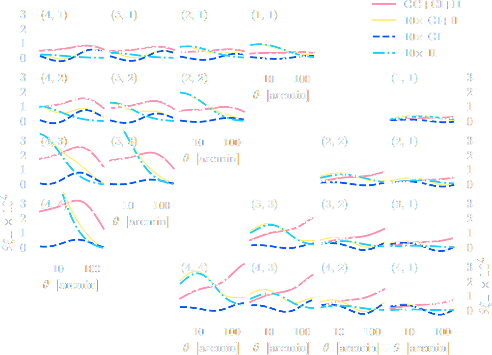
DES Y3 Cosmic Shear data vector
$\Longrightarrow$ Can we find non-Gaussian information that is not affected by baryons?
takeways
-
SBI automatizes inference over
numerical simulators.
- Turns both summary extraction and inference problems into an optimization problems
- Deep learning allows us to solve that problem!
-
In the context of upcoming surveys, this techniques provides
many advantages:
- Amortized inference: near instantaneous parameter inference, extremely useful for time-domain.
- Optimal information extraction: no longer need for restrictive modeling assumptions needed to obtain tractable likelihoods.
Will we be able to exploit all of the information content of
LSST, Euclid, DESI?
$\Longrightarrow$ Not rightaway, but it is not the fault of Deep
Learning!
- Deep Learning has redefined the limits of our statistical tools, creating additional demand on the accuracy of simulations far beyond the power spectrum.
- Neural compression methods have the downside of being opaque. It is much harder to detect unknown systematics.
- We will need a significant number of large volume, high resolution simulations.
Extra slides: Examples of other applications
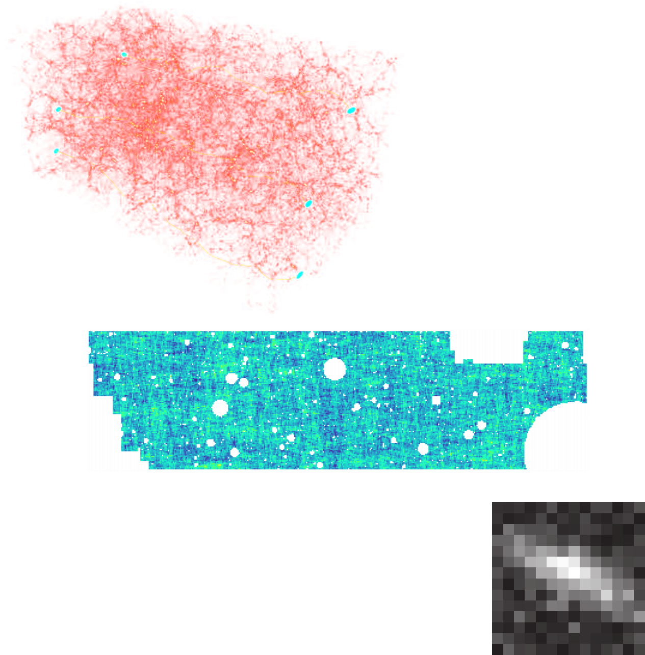
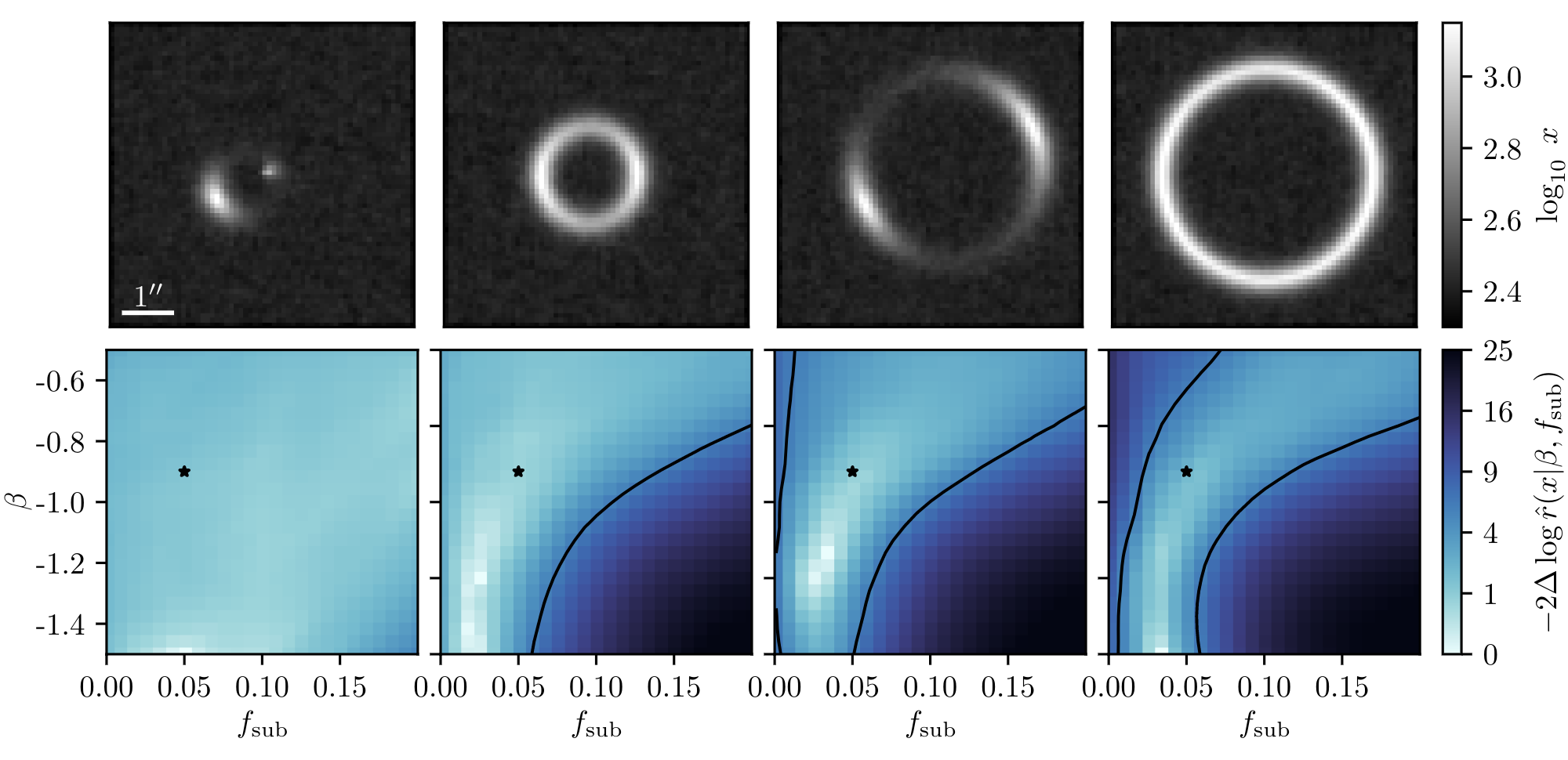
Example of application: Constraining Dark Matter Substructures
Brehmer, Mishra-Sharma, Hermans, Louppe, Cranmer (2019) 

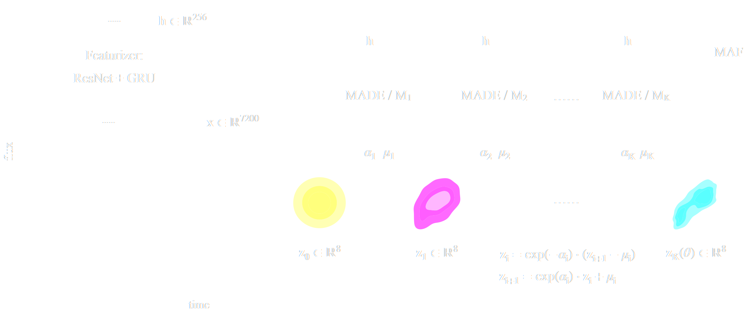
Example of application: Infering Microlensing Event Parameters
Zhang, Bloom, Gaudi, Lanusse, Lam, Lu (2021)