Merging deep learning with physical models
for the analysis of modern cosmological surveys
François Lanusse

slides at eiffl.github.io/talks/LIneA2020
the Rubin Observatory Legacy Survey of Space and Time
- 1000 images each night, 15 TB/night for 10 years
- 18,000 square degrees, observed once every few days
- Tens of billions of objects, each one observed $\sim1000$ times
Previous generation survey: SDSS
Image credit: Peter Melchior
Current generation survey: DES
Image credit: Peter Melchior
LSST precursor survey: HSC
Image credit: Peter Melchior
The challenges of modern surveys
$\Longrightarrow$ Modern surveys will provide large volumes of high quality data
A Blessing
- Unprecedented statistical power
- Great potential for new discoveries
A Curse
- Existing methods are reaching their limits at every step of the science analysis
- Control of systematics is paramount
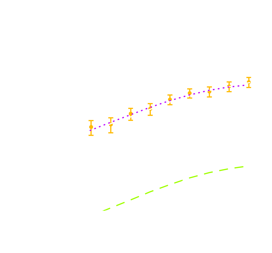
LSST forecast on dark energy parameters
![]()
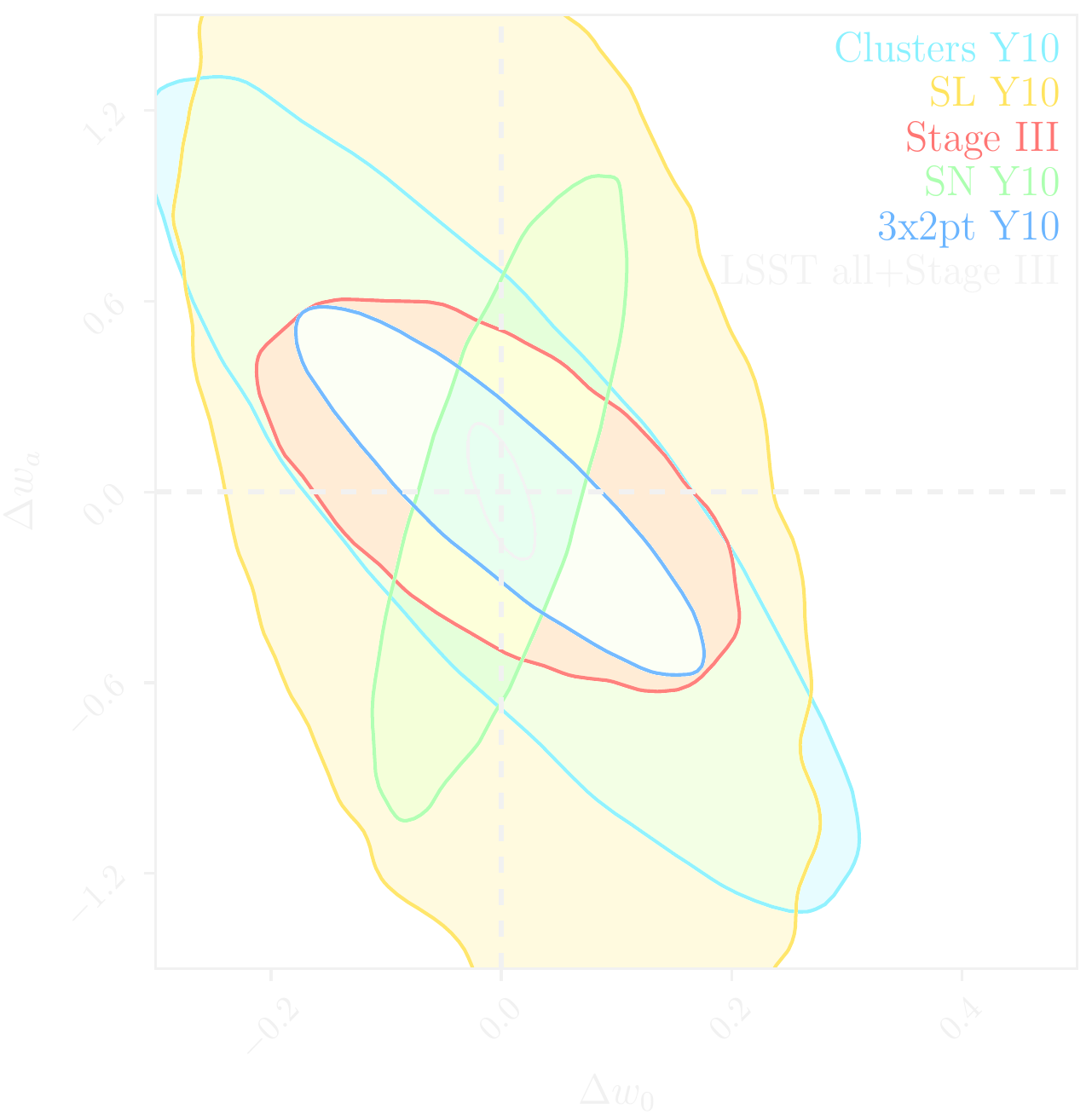
$\Longrightarrow$ Dire need for novel analysis techniques to fully realize the potential of modern surveys:
Outline of this talk
How can we merge Deep Learning and Physical Models to help us make sense
of increasingly complex data?
- Generative Models for Galaxy Image Simulations
- Data-driven priors for Astronomical Inverse Problems
- Differentiable models of the Large Scale Structure
Generative Models for Galaxy Image Simulation
Work in collaboration with
Rachel Mandelbaum, Siamak Ravanbakhsh, Barnabas Poczos, Peter Freeman
Lanusse et al., in prep
Ravanbakhsh, Lanusse, et al. (2017)
Ravanbakhsh, Lanusse, et al. (2017)
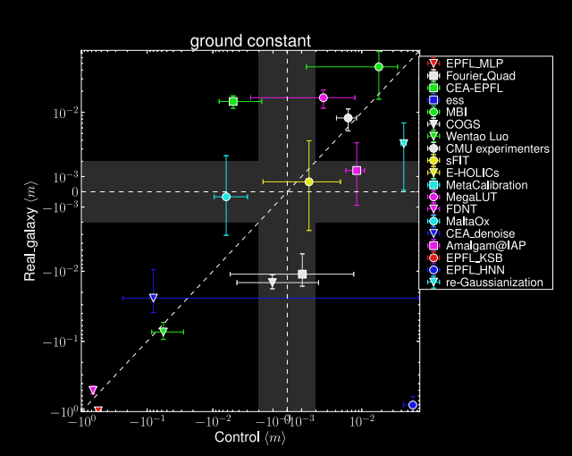
The weak lensing shape measurement problem
Shape measurement biases
$$ < e > = \ (1 + m) \ \gamma \ + \ c $$
- Can be calibrated on image simulations
- How complex do the simulations need to be?
Impact of galaxy morphology
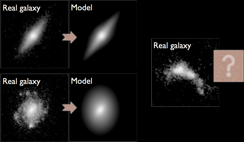
Mandelbaum, et al. (2013), Mandelbaum, et al. (2014)
The need for data-driven generative models
- Lack or inadequacy of physical model
- Extremely computationally expensive simulations
Can we learn a model for the signal from the data itself?
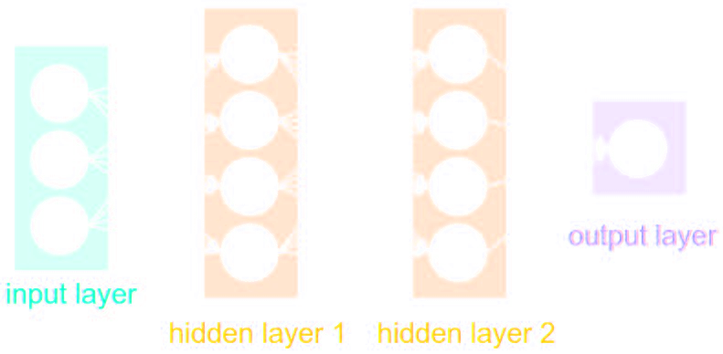
The evolution of generative models
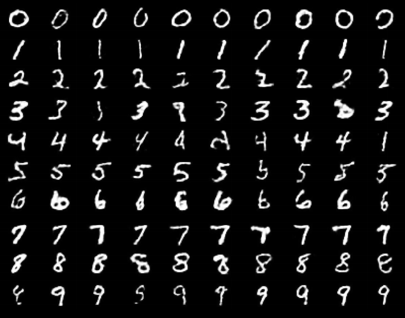
- Deep Belief Network
(Hinton et al. 2006) - Variational AutoEncoder
(Kingma & Welling 2014) - Generative Adversarial Network
(Goodfellow et al. 2014) - Wasserstein GAN
(Arjovsky et al. 2017)
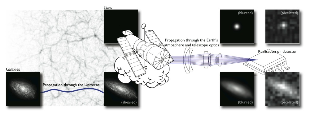
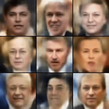
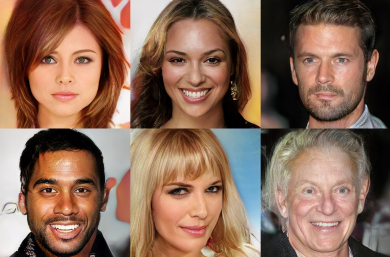
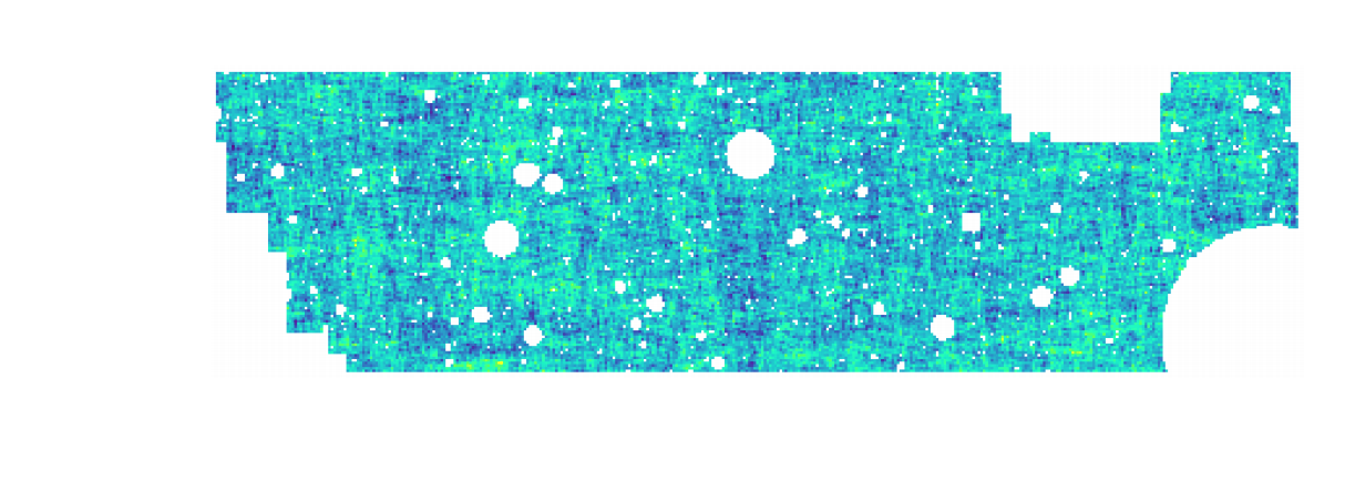
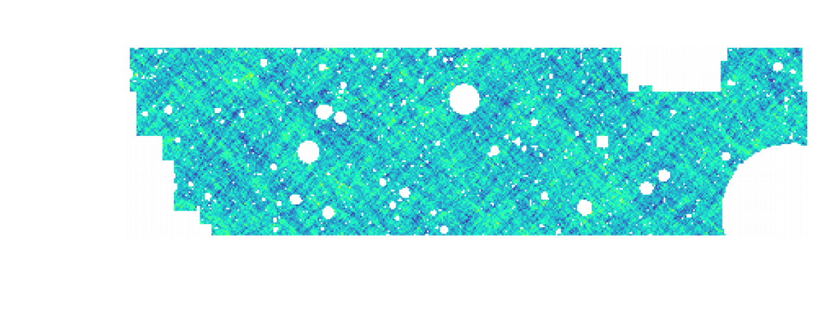
Complications specific to astronomical images: spot the differences!
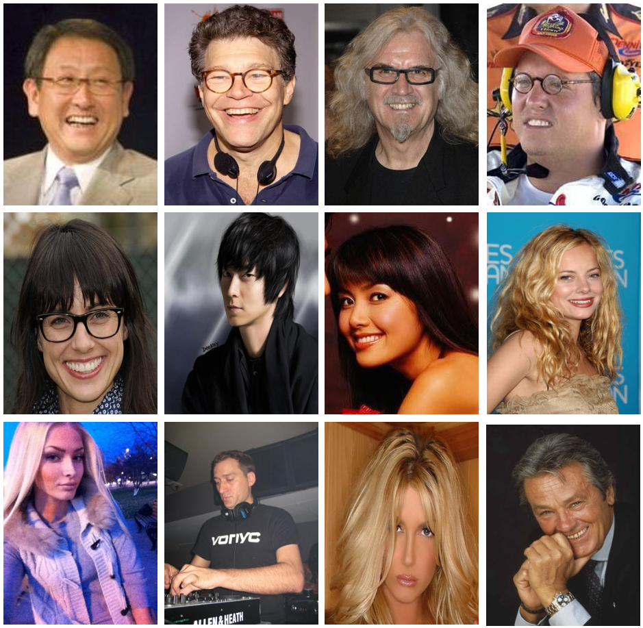
CelebA
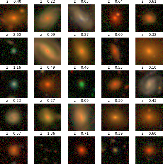
HSC PDR-2 wide
- There is noise
- We have a Point Spread Function
A Physicist's approach: let's build a model

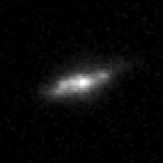
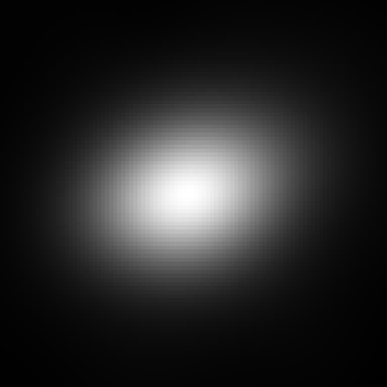
$\longrightarrow$
$g_\theta$
$g_\theta$
$\longrightarrow$
PSF
PSF
$\longrightarrow$
Pixelation
Pixelation
$\longrightarrow$
Noise
Noise
Probabilistic model
$$ x \sim ? $$
$$ x \sim \mathcal{N}(z, \Sigma) \quad z \sim ? $$
latent $z$ is a denoised galaxy image
latent $z$ is a denoised galaxy image
$$ x \sim \mathcal{N}( \mathbf{P} z, \Sigma) \quad z \sim ?$$
latent $z$ is a super-resolved and denoised galaxy image
latent $z$ is a super-resolved and denoised galaxy image
$$ x \sim \mathcal{N}( \mathbf{P} (\Pi \ast z), \Sigma) \quad z \sim ? $$
latent $z$ is a deconvolved, super-resolved, and denoised galaxy image
latent $z$ is a deconvolved, super-resolved, and denoised galaxy image
$$ x \sim \mathcal{N}( \mathbf{P} (\Pi \ast g_\theta(z)), \Sigma) \quad z \sim \mathcal{N}(0, \mathbf{I}) $$
latent $z$ is a Gaussian sample
$\theta$ are parameters of the model
latent $z$ is a Gaussian sample
$\theta$ are parameters of the model
$\Longrightarrow$ Decouples the morphology model from the observing conditions.
How to train your dragon model
- Training the generative amounts to finding $\theta_\star$ that
maximizes the marginal likelihood of the model:
$$p_\theta(x | \Sigma, \Pi) = \int \mathcal{N}( \Pi \ast g_\theta(z), \Sigma) \ p(z) \ dz$$
$\Longrightarrow$ This is generally intractable
- Efficient training of parameter $\theta$ is made possible by Amortized Variational Inference.
Auto-Encoding Variational Bayes (Kingma & Welling, 2014)
- We introduce a parametric distribution $q_\phi(z | x, \Pi, \Sigma)$ which aims to model the posterior $p_{\theta}(z | x, \Pi, \Sigma)$.
- Working out the KL divergence between these two distributions leads to: $$\log p_\theta(x | \Sigma, \Pi) \quad \geq \quad - \mathbb{D}_{KL}\left( q_\phi(z | x, \Sigma, \Pi) \parallel p(z) \right) \quad + \quad \mathbb{E}_{z \sim q_{\phi}(. | x, \Sigma, \Pi)} \left[ \log p_\theta(x | z, \Sigma, \Pi) \right]$$ $\Longrightarrow$ This is the Evidence Lower-Bound, which is differentiable with respect to $\theta$ and $\phi$.
The famous Variational Auto-Encoder
$$\log p_\theta(x| \Sigma, \Pi ) \geq - \underbrace{\mathbb{D}_{KL}\left( q_\phi(z | x, \Sigma, \Pi) \parallel p(z) \right)}_{\mbox{code regularization}} + \underbrace{\mathbb{E}_{z \sim q_{\phi}(. | x, \Sigma, \Pi)} \left[ \log p_\theta(x | z, \Sigma, \Pi) \right]}_{\mbox{reconstruction error}} $$
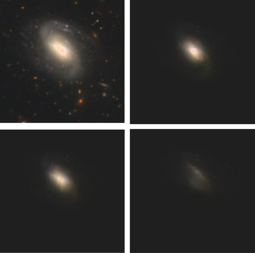
Illustration on HST/ACS COSMOS images

Fitting observations with VAE and Bulge+Disk parametric model.
- Training set: GalSim COSMOS HST/ACS postage stamps
- 80,000 deblended galaxies from I < 25.2 sample
- Drawn on 128x128 stamps at 0.03 arcsec resolution
- Each stamp comes with:
- PSF
- Noise power spectrum
- Bulge+Disk parametric fit
- Auto-Encoder model:
- Deep residual autoencoder:
7 stages of 2 resnet blocs each - Dense bottleneck of size 32.
- Outputs positive, noiseless, deconvolved, galaxy surface brightness.
- Deep residual autoencoder:
Flow-VAE samples


Testing conditional sampling


$\Longrightarrow$ We can successfully condition galaxy generation.
Testing galaxy morphologies

Takeaway message
- We have combined physical and deep learning components to model
observed noisy and PSF-convoled galaxy images.
$\Longrightarrow$ This framework can handle multi-band, multi-resolution, multi-instrument data. - We demonstrate conditional sampling of galaxy light profiles
$\Longrightarrow$ Image simulation can be combined with larger survey simulation efforts, e.g. LSST DESC DC2
GalSim Hub

- Framework for sampling from deep generative models directly from within GalSim.
- Go check out the alpha version: https://github.com/McWilliamsCenter/galsim_hub
Data-driven priors for astronomical inverse problems
Work in collaboration with
Peter Melchior, Fred Moolekamp, Remy Joseph
Lanusse, Melchior, Moolekamp (2019)
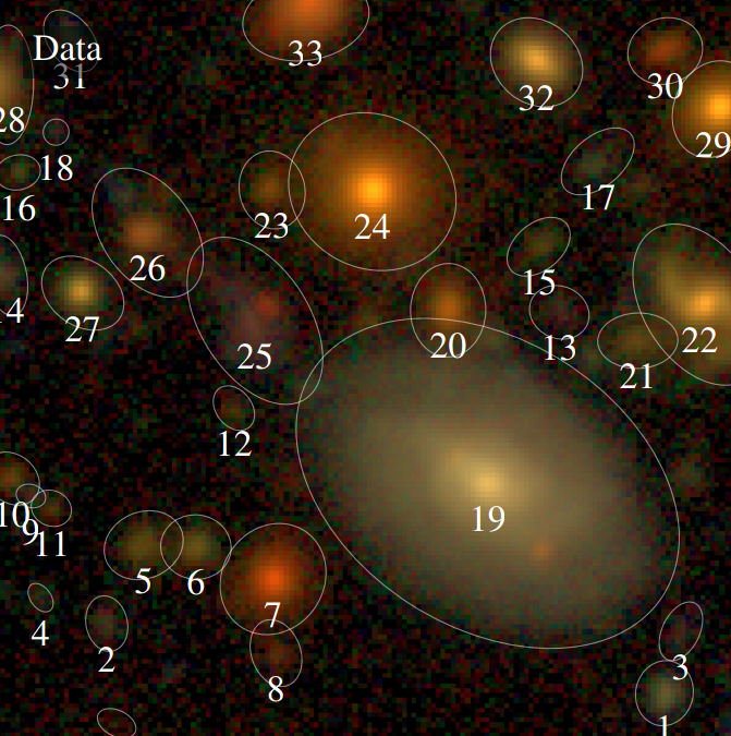
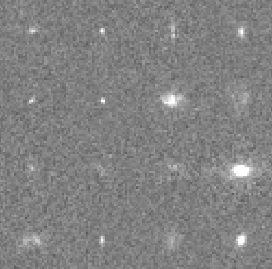
The challenge of galaxy blending
Bosch et al. 2017
- In HSC over 60% of all galaxies are blended
- Important impact on our main cosmological probes
- Current generation of deblenders does not meet our target requirements
- Existing methods rely on simple assumptions about galaxy profiles, like symmetry or monotonicity
Deblending is an ill-posed inverse problem, akin to Blind Source Separation. The is no single solution.
$\Longrightarrow$ Intuitively, the key will be to leverage an understanding of how individual galaxies look like.
$\Longrightarrow$ Intuitively, the key will be to leverage an understanding of how individual galaxies look like.
A Bayesian view of the problem
$\boxed{y = \mathbf{A}x + n}$
$$ p(x | y) \propto p(y | x) \ p(x) $$
- $p(y | x)$ is the data likelihood, which contains the physics
- $p(x)$ is our prior knowledge on the solution.
With these concepts in hand, we want to estimate the Maximum A Posteriori solution:
$$\hat{x} = \arg\max\limits_x \ \log p(y \ | \ x) + \log p(x)$$
For instance, if $n$ is Gaussian, $\hat{x} = \arg\max\limits_x \ - \frac{1}{2} \parallel y - \mathbf{A} x \parallel_{\mathbf{\Sigma}}^2 + \log p(x)$
$$\hat{x} = \arg\max\limits_x \ \log p(y \ | \ x) + \log p(x)$$
For instance, if $n$ is Gaussian, $\hat{x} = \arg\max\limits_x \ - \frac{1}{2} \parallel y - \mathbf{A} x \parallel_{\mathbf{\Sigma}}^2 + \log p(x)$
How do you choose the prior ?
Classical examples of signal priors
Sparse
![]()
$$ \log p(x) = \parallel \mathbf{W} x \parallel_1 $$
$$ \log p(x) = \parallel \mathbf{W} x \parallel_1 $$
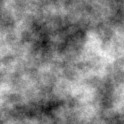
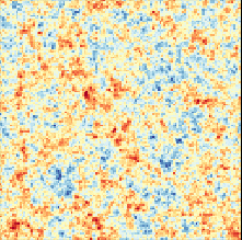
Gaussian
![]() $$ \log p(x) = x^t \mathbf{\Sigma^{-1}} x $$
$$ \log p(x) = x^t \mathbf{\Sigma^{-1}} x $$
 $$ \log p(x) = x^t \mathbf{\Sigma^{-1}} x $$
Total Variation
![]() $$ \log p(x) = \parallel \nabla x \parallel_1 $$
$$ \log p(x) = \parallel \nabla x \parallel_1 $$
But what about this?
PixelCNN: Likelihood-based Autoregressive generative model
Models the probability $p(x)$ of an image $x$ as:
$$ p_{\theta}(x) = \prod_{i=0}^{n} p_{\theta}(x_i | x_{i-1} \ldots x_0) $$
- $p_\theta(x)$ is explicit! We get a number out.
- We can train the model to learn a distribution of isolated galaxy images.
- We can then evaluate its gradient $\frac{\color{orange} d \color{orange}\log \color{orange}p\color{orange}(\color{orange}x\color{orange})}{\color{orange} d \color{orange}x}$.
van den Oord et al. 2016
- Check out another application of these models to discrimination between real (SDSS) and simulated (Illustris TNG) galaxy populations: Zanisi, Huertas-Company, Lanusse et al. 2020 arXiv:2007.00039
The Scarlet algorithm: deblending as an optimization problem
Melchior et al. 2018
$$ \mathcal{L} = \frac{1}{2} \parallel \mathbf{\Sigma}^{-1/2} (\ Y - P \ast A S \ ) \parallel_2^2 - \sum_{i=1}^K \log p_{\theta}(S_i) + \sum_{i=1}^K g_i(A_i) + \sum_{i=1}^K f_i(S_i)$$
Where for a $K$ component blend:
- $P$ is the convolution with the instrumental response
- $A_i$ are channel-wise galaxy SEDs, $S_i$ are the morphology models
- $\mathbf{\Sigma}$ is the noise covariance
- $\log p_\theta$ is a PixelCNN prior
- $f_i$ and $g_i$ are arbitrary additional non-smooth consraints, e.g. positivity, monotonicity...
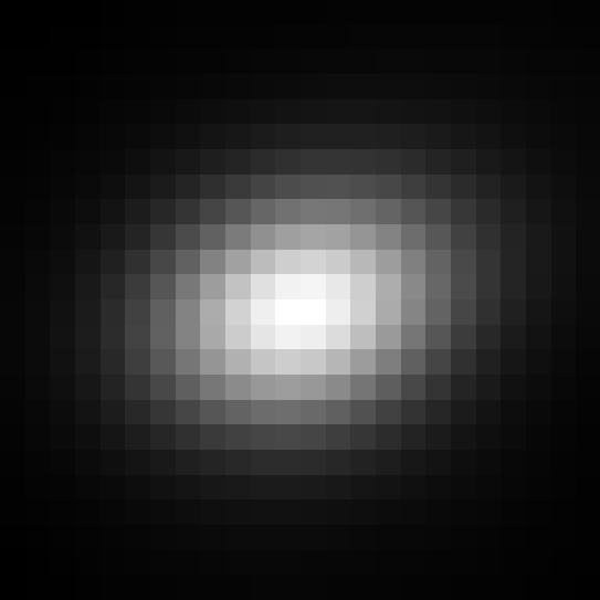
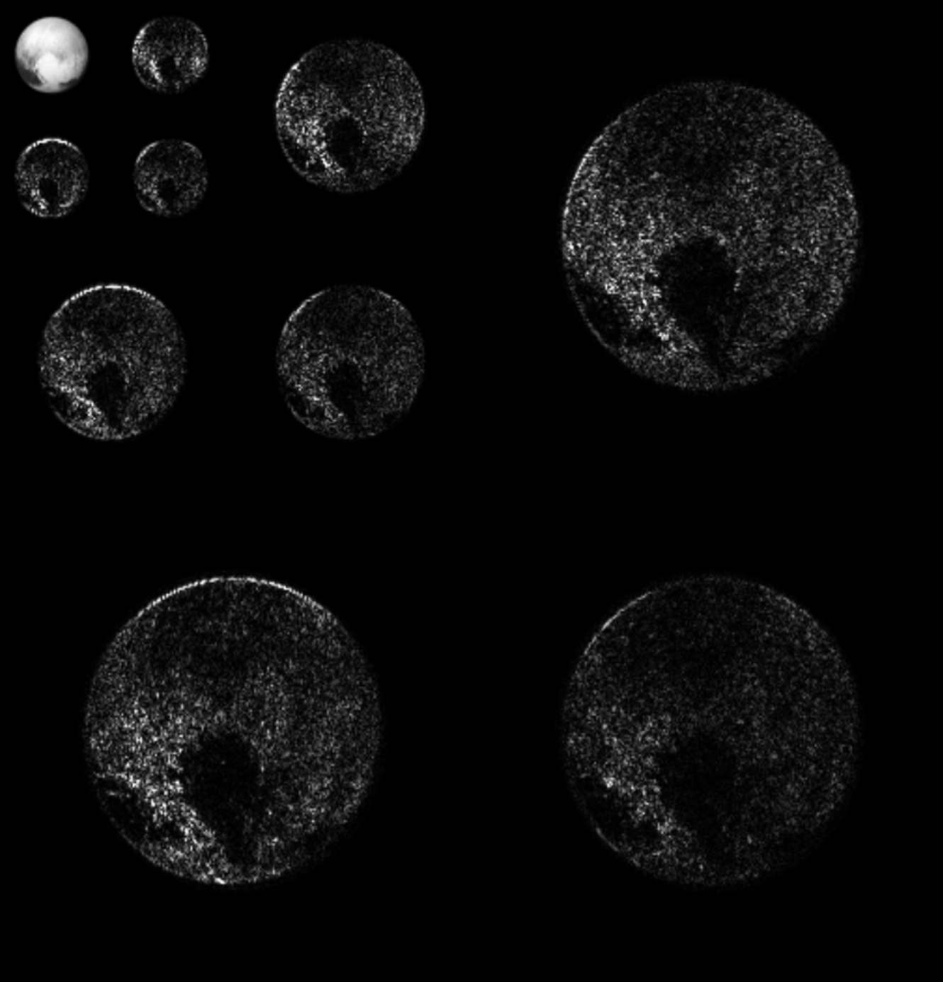
Training the morphology prior
Postage stamps of isolated COSMOS galaxies used for training, at WFIRST resolution and fixed fiducial PSF
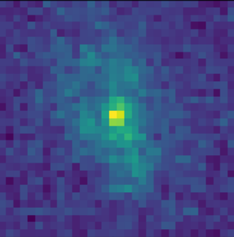
isolated galaxy
![]() $\log p_\theta(x) = 3293.7$
$\log p_\theta(x) = 3293.7$
 $\log p_\theta(x) = 3293.7$
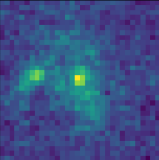
artificial blend
![]() $\log p_\theta(x) = 3100.5 $
$\log p_\theta(x) = 3100.5 $
 $\log p_\theta(x) = 3100.5 $
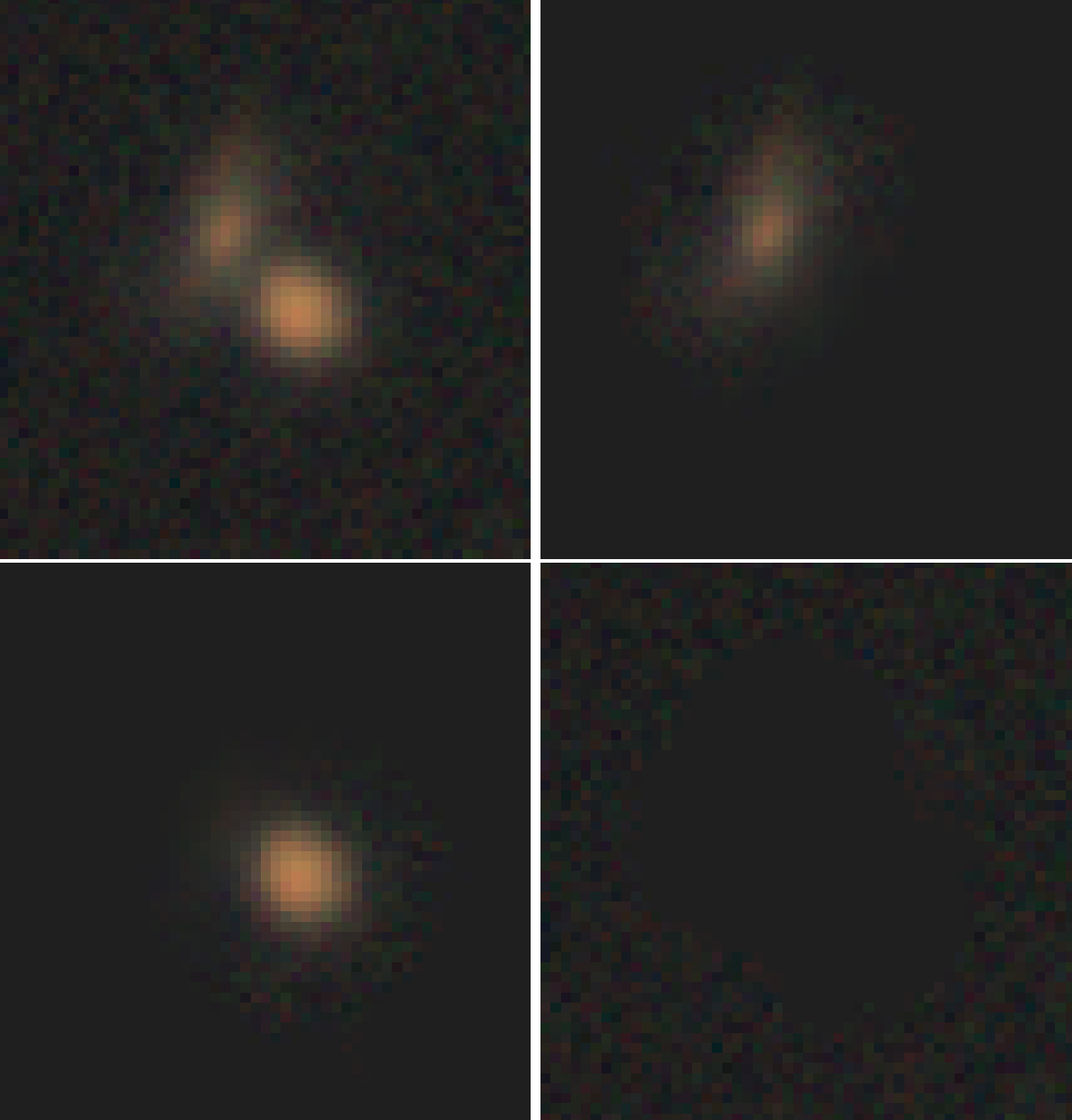
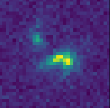
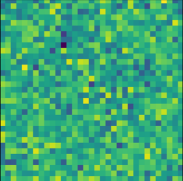
Scarlet in action
Input blend
![]()
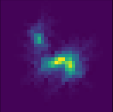
Solution
![]()
![]()
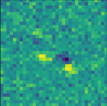
Residuals
![]()
![]()
- Classic priors (monotonicity, symmetry).
- Deep Morphology prior.
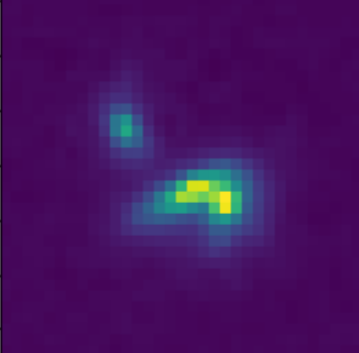
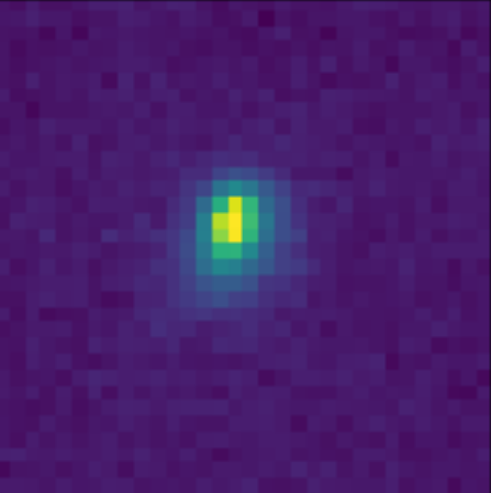
True Galaxy
![]()
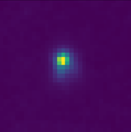
Deep Morphology Prior Solution
![]()
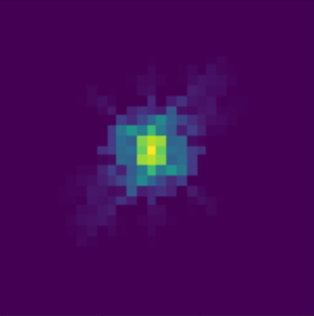
Monotonicity + Symmetry Solution
![]()
Extending to multi-band images

Takeaway message
- We have introduce an hybrid physical/deep learning model for inverse problems
- Incorporate prior astrophysical knowledge as a data-driven prior
- Interpretable in terms of physical components of the astronomical scene
- Can accomodate different observing conditions and instruments
$\Longrightarrow$ For instance, for the joint modeling of LSST/Euclid data
Differentiable models of the Large-Scale Structure
Work in collaboration with
Chirag Modi, Uroš Seljak

Modi, Lanusse, Seljak, et al., in prep
Modi, et al. (2018)
Modi, et al. (2018)
traditional cosmological inference
HSC cosmic shear power spectrum
HSC Y1 constraints on $(S_8, \Omega_m)$
(Hikage,..., Lanusse, et al. 2018)
- Measure the ellipticity $\epsilon = \epsilon_i + \gamma$ of all galaxies
$\Longrightarrow$ Noisy tracer of the weak lensing shear $\gamma$ - Compute summary statistics based on 2pt functions,
e.g. the power spectrum - Run an MCMC to recover a posterior on model parameters, using an analytic likelihood $$ p(\theta | x ) \propto \underbrace{p(x | \theta)}_{\mathrm{likelihood}} \ \underbrace{p(\theta)}_{\mathrm{prior}}$$
Main limitation: the need for an explicit likelihood
We can only compute the likelihood for simple summary statistics and on large scales
$\Longrightarrow$ We are dismissing most of the information!
A different road: forward modeling
- Instead of trying to analytically evaluate the likelihood, let us build a forward model of the observables.
- Each component of the model is now tractable, but at the cost of a large number of latent variables.
$\Longrightarrow$ How to peform efficient inference in this large number of dimensions?
- A non-exhaustive list of methods:
- Hamiltonian Monte-Carlo
- Variational Inference
- MAP+Laplace
- Gold Mining
- Dimensionality reduction by Fisher-Information Maximization
What do they all have in common?
-> They require fast, accurate, differentiable forward simulations
-> They require fast, accurate, differentiable forward simulations
(Schneider et al. 2015)
How do we simulate the Universe in a fast and differentiable way?
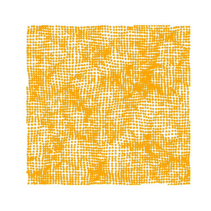
Forward Models in Cosmology
 Linear Field
 Final Dark Matter
$\longrightarrow$
N-body simulations
N-body simulations
the Fast Particle-Mesh scheme for N-body simulations
The idea: approximate gravitational forces by esimating densities on a grid.- The numerical scheme:
- Estimate the density of particles on a mesh
=> compute gravitational forces by FFT - Interpolate forces at particle positions
- Update particle velocity and positions, and iterate
- Estimate the density of particles on a mesh
- Fast and simple, at the cost of approximating short range interactions.
$\Longrightarrow$ Only a series of FFTs and interpolations.
introducing FlowPM: Particle-Mesh Simulations in TensorFlow

											                  import tensorflow as tf
											                  import flowpm
											                  # Defines integration steps
											                  stages = np.linspace(0.1, 1.0, 10, endpoint=True)

											                  initial_conds = flowpm.linear_field(32,        # size of the cube
											                                                      100,       # Physical size
											                                                      ipklin,    # Initial powerspectrum
											                                                      batch_size=16)

											                  # Sample particles and displace them by LPT
											                  state = flowpm.lpt_init(initial_conds, a0=0.1)

											                  # Evolve particles down to z=0
											                  final_state = flowpm.nbody(state, stages, 32)

											                  # Retrieve final density field
											                  final_field = flowpm.cic_paint(tf.zeros_like(initial_conditions),
											                                                 final_state[0])

											                  with tf.Session() as sess:
											                      sim = sess.run(final_field)
- Seamless interfacing with deep learning components
- Mesh TensorFlow implementation for distribution on supercomputers
Forward Models in Cosmology
Linear Field
Final Dark Matter
 Dark Matter Halos
 Galaxies
$\longrightarrow$
N-body simulations
FlowPM
N-body simulations
FlowPM
$\longrightarrow$
Group Finding
algorithms
Group Finding
algorithms
$\longrightarrow$
Semi-analytic &
distribution models
Semi-analytic &
distribution models
Example of Extending Dark Matter Simulations with Deep Learning

$\longrightarrow$


Modi et al. 2018
Takeaway message
- We are combining physical and deep learning components to model
the Large-Scale Structure in a fast and differentiable way.
$\Longrightarrow$ This is a necessary backbone for large scale simulation-based inference. - We are demonstrating that large-scale simulations can be
implemented in distributed autodiff frameworks.
$\Longrightarrow$ We hope that this will one day become the norm.
Check out this blogpost to learn more
https://blog.tensorflow.org/2020/03/simulating-universe-in-tensorflow.html
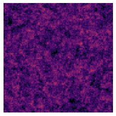
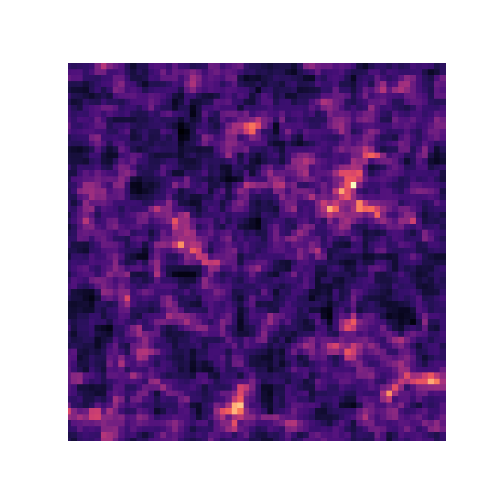
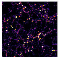
![]()
True initial conditions
$z_0$
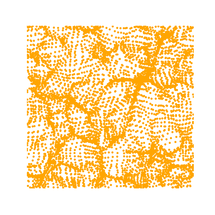
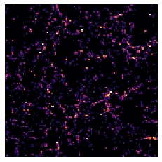
![]()
Reconstructed initial conditions $z$
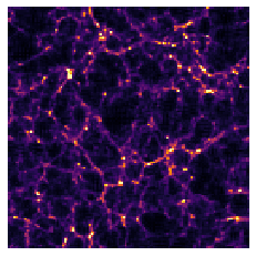
![]()
Reconstructed dark matter distribution $x = f(z)$
![]()
Data
$x_{DM} = f(z_0)$
https://blog.tensorflow.org/2020/03/simulating-universe-in-tensorflow.html
True initial conditions
$z_0$
Reconstructed initial conditions $z$
Reconstructed dark matter distribution $x = f(z)$
Data
$x_{DM} = f(z_0)$
Conclusion
Conclusion
What can be gained by merging Deep Learning and Physical Models?
- Complement known physical models with data-driven components
- Learn galaxy morphologies from noisy and PSF-convolved data, for simulation purposes.
- Use data-driven model as prior for solving inverse problems such as deblending or deconvolution.
- Differentiable physical models for fast inference
- We are developing fast and distributed N-body simulations in TensorFlow.
- Even analytic cosmological computations can benefit from differentiability.
https://github.com/DifferentiableUniverseInitiative/jax_cosmo
Advertisement:
- Differentiable Universe Initiative (gitter.im/DifferentiableUniverseInitiative): Group of people interested in making everything differentiable! join the conversation :-)
Thank you !