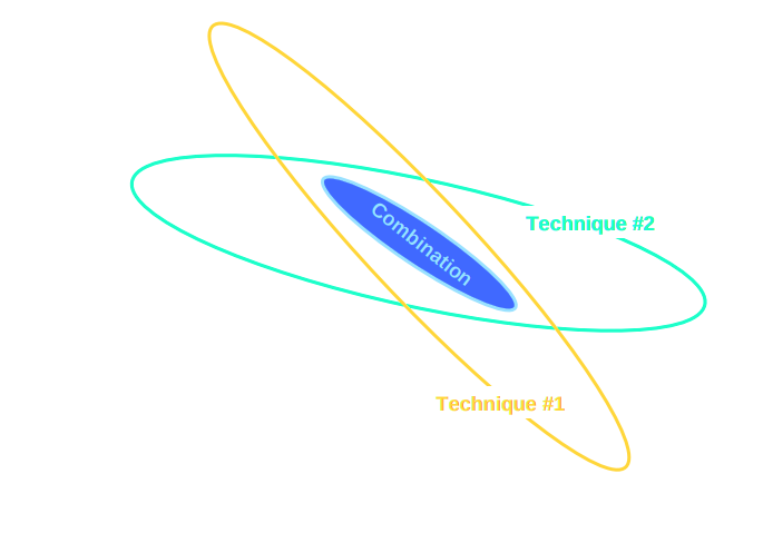
What are cosmologists trying to go after with galaxy surveys?
We have been dreaming about these surveys for 20 years!
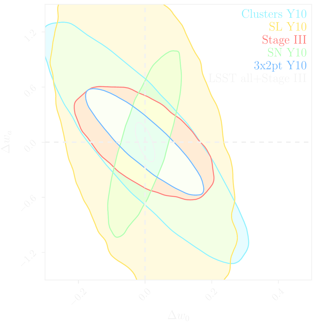
Albrecht et al. (2006)
LSST forecast on dark energy parameters
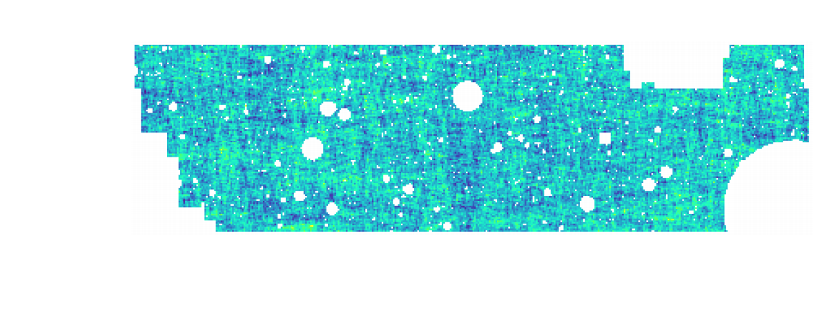
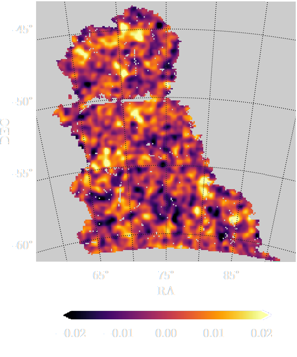
Image credit: N. Jeffrey / DES Collaboration
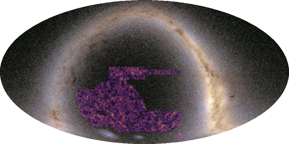
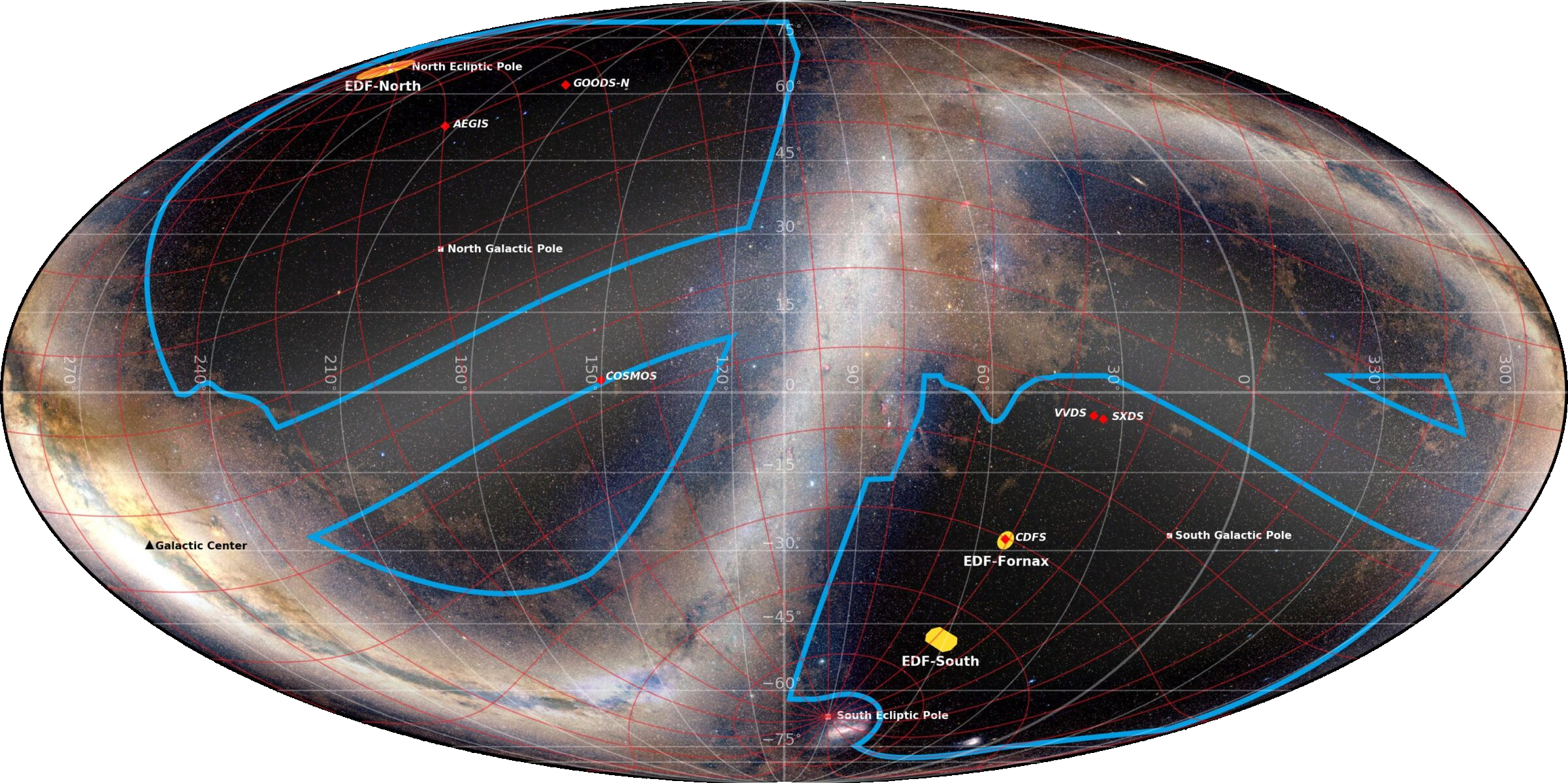
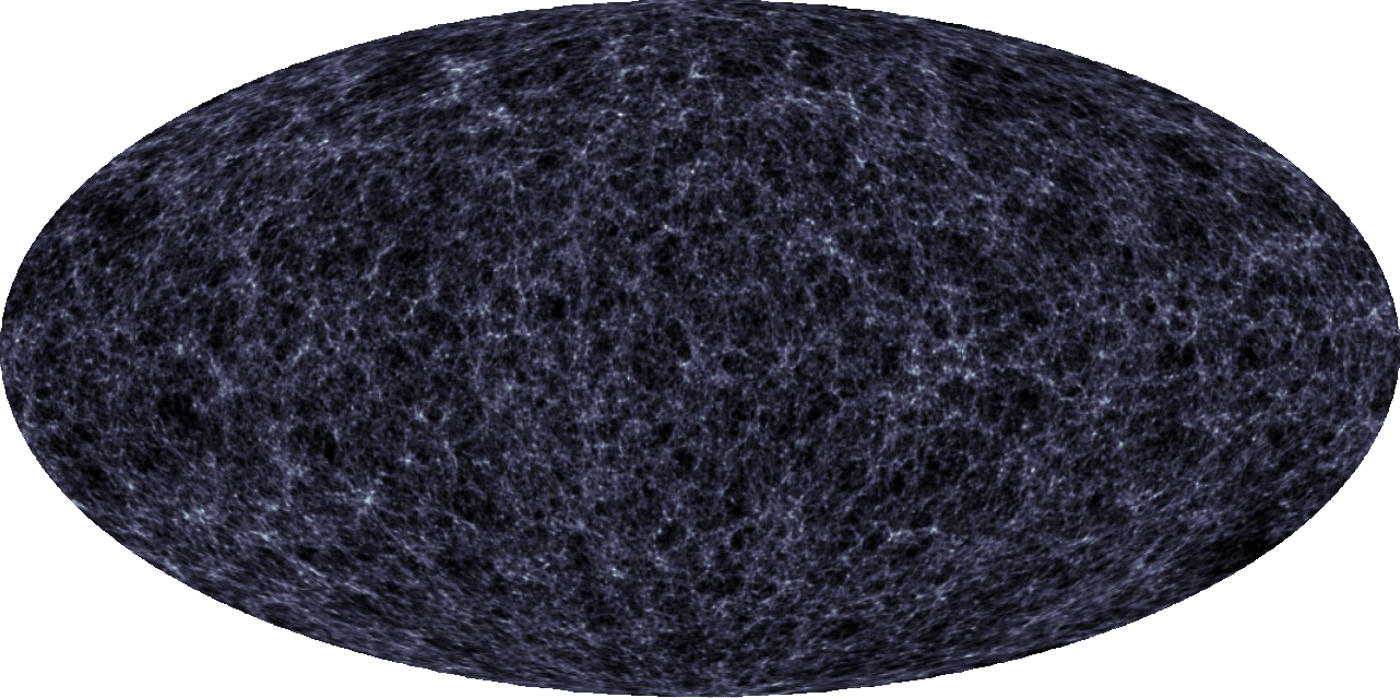
Image credit: Euclid Consortium / Planck Collaboration / A. Mellinger
Stage II: SDSS
Image credit: Peter Melchior
Stage III: DES
Image credit: Peter Melchior
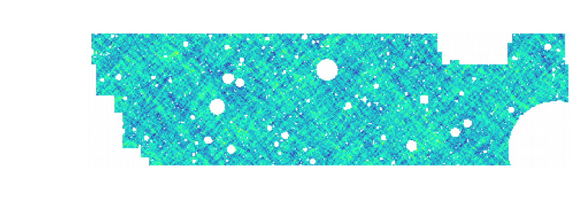
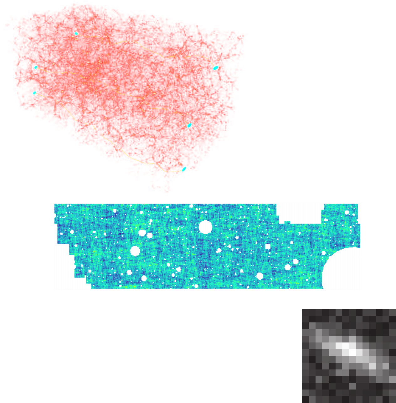
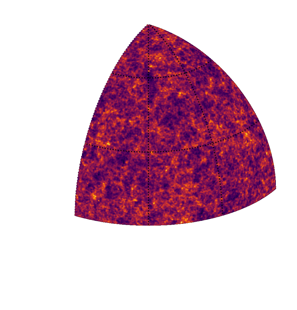
Stage IV: Rubin Observatory LSST (HSC)
Image credit: Peter Melchior
Euclid Q1 Data Release: April 2025
Image credit: ESA/Euclid/Euclid Consortium/NASA
Image processing by J.-C. Cuillandre, E. Bertin, G. Anselmi
the Vera C. Rubin Observatory Legacy Survey of Space and Time
1000 images each night, 15 TB/night for 10 years
18,000 square degrees, observed once every few days
Tens of billions of objects, each one observed $\sim1000$ times
Rubin First Look, Monday June 23rd!
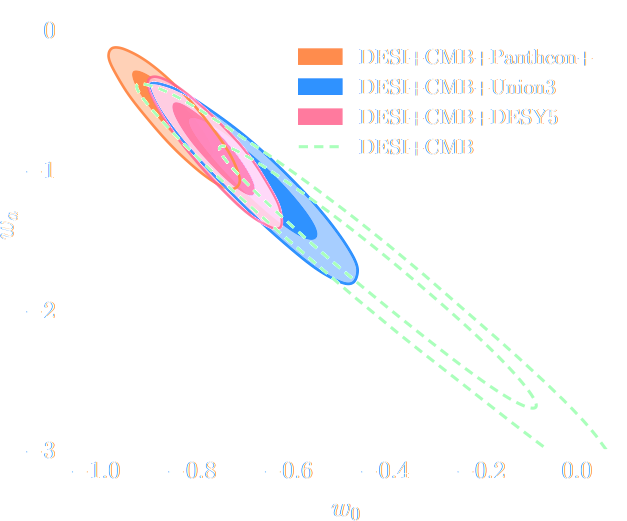
Dark Energy Spectroscopic Instrument (DESI) is teasing us with new tensions!
DESI Collaboration (2025)
Ok, exciting, but where is the AI you promised???
What does a conventional cosmological analysis look like?
The limits of traditional cosmological inference
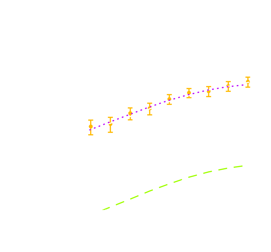
HSC cosmic shear power spectrum
HSC Y1 constraints on $(S_8, \Omega_m)$
(Hikage et al. 2018)
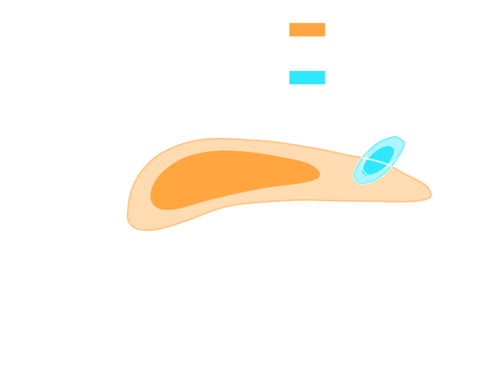
Measure the ellipticity $\epsilon = \epsilon_i + \gamma$ of all galaxies
$\Longrightarrow$ Noisy tracer of the weak lensing shear $\gamma$
Compute summary statistics based on 2pt functions, e.g. the power spectrum
Run an MCMC to recover a posterior on model parameters, using an analytic likelihood
$$ p(\theta | x ) \propto \underbrace{p(x | \theta)}_{\mathrm{likelihood}} \ \underbrace{p(\theta)}_{\mathrm{prior}}$$
Main limitation: the need for an explicit likelihood
We can only compute from theory the likelihood for simple summary statistics and on large scales
$\Longrightarrow$ We are dismissing a significant fraction of the information!
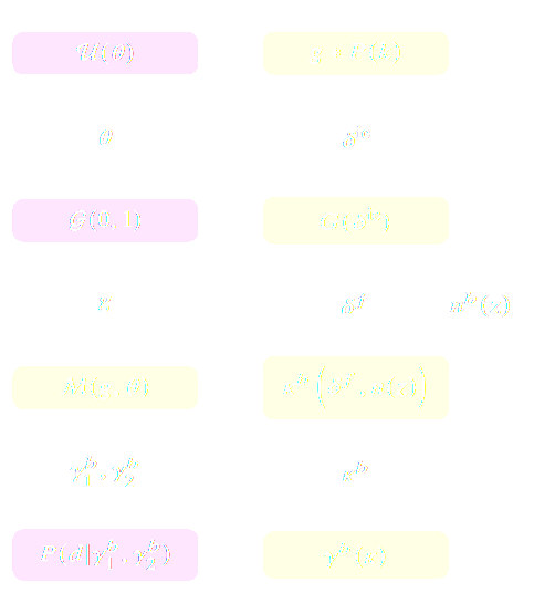
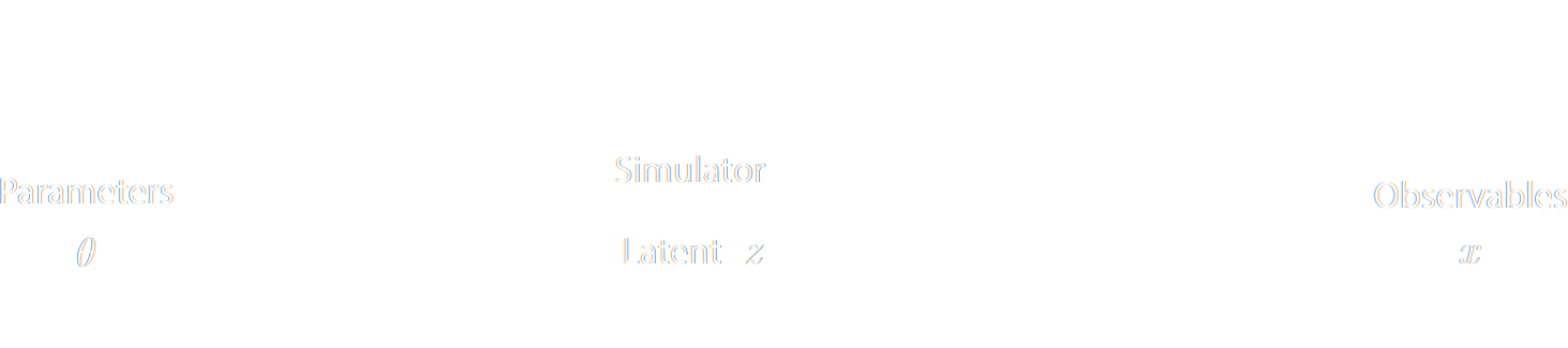
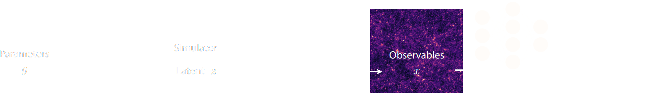
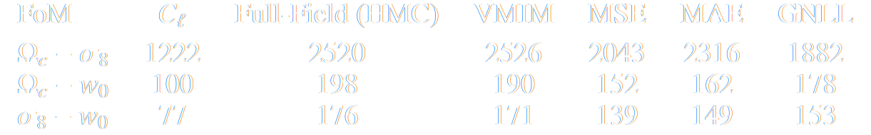
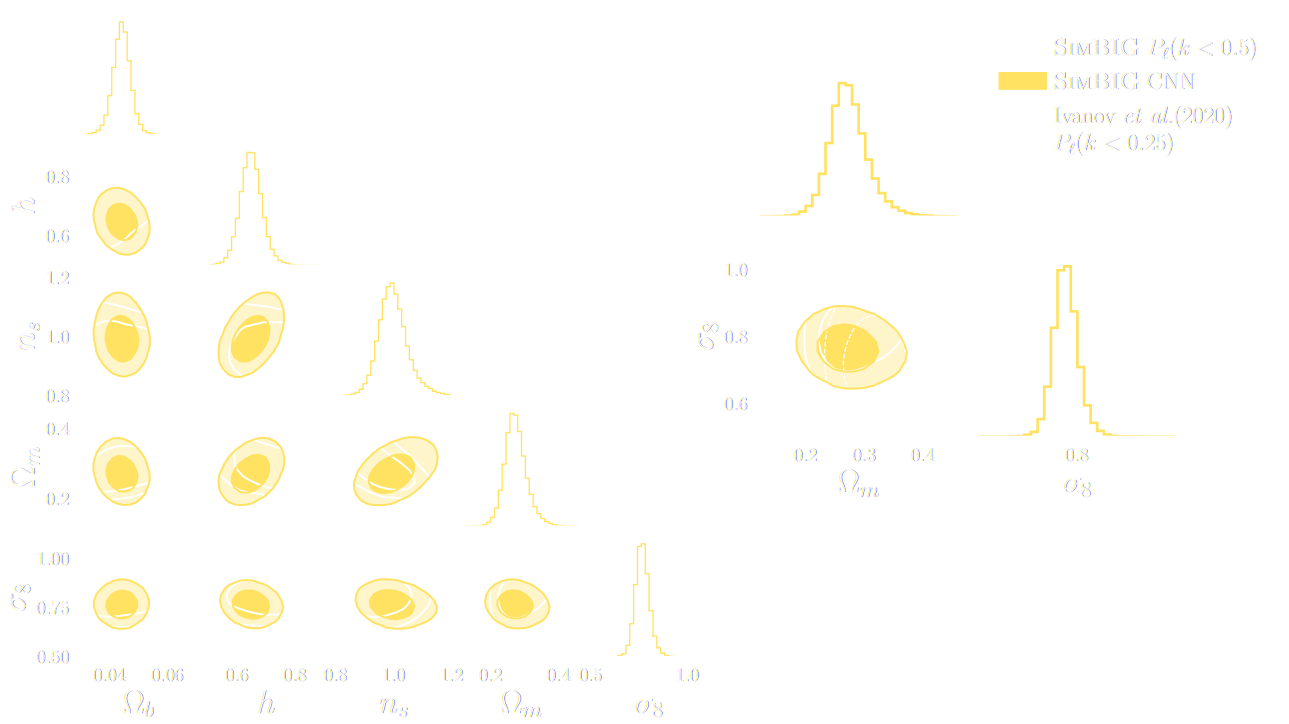
Full-Field Simulation-Based Inference
Instead of trying to analytically evaluate the likelihood of
sub-optimal summary statistics, let us build a forward model of the full observables.
$\Longrightarrow$ The simulator becomes the physical model.
Each component of the model is now tractable, but at the
cost of a large number of latent variables.
Benefits of a forward modeling approach
Fully exploits the information content of the data
(aka "full field inference").
Easy to incorporate systematic effects.
Easy to combine multiple cosmological probes by joint simulations.
(Porqueres et al. 2021)
Just as a reminder, why is it classicaly hard to do simulation-based inference?
The Challenge of Simulation-Based Inference
$$ p(x|\theta) = \int p(x, z | \theta) dz = \int p(x | z, \theta) p(z | \theta) dz $$
Where $z$ are stochastic latent variables of the simulator.
$\Longrightarrow$ This marginal likelihood is intractable!
How to perform inference over forward simulation models?
Implicit Inference: Treat the simulator as a black-box with only the ability to sample from the joint distribution
$$(x, \theta) \sim p(x, \theta)$$
a.k.a.
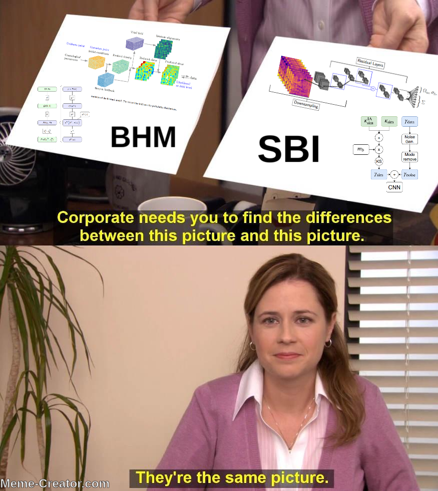
Simulation-Based Inference (SBI)
Likelihood-free inference (LFI)
Approximate Bayesian Computation (ABC)
Explicit Inference: Treat the simulator as a probabilistic model and perform inference over the joint posterior
$$p(\theta, z | x) \propto p(x | z, \theta) p(z, \theta) p(\theta) $$
a.k.a.
Bayesian Hierarchical Modeling (BHM)
$\Longrightarrow$ For a given simulation model, both methods should converge to the same posterior!
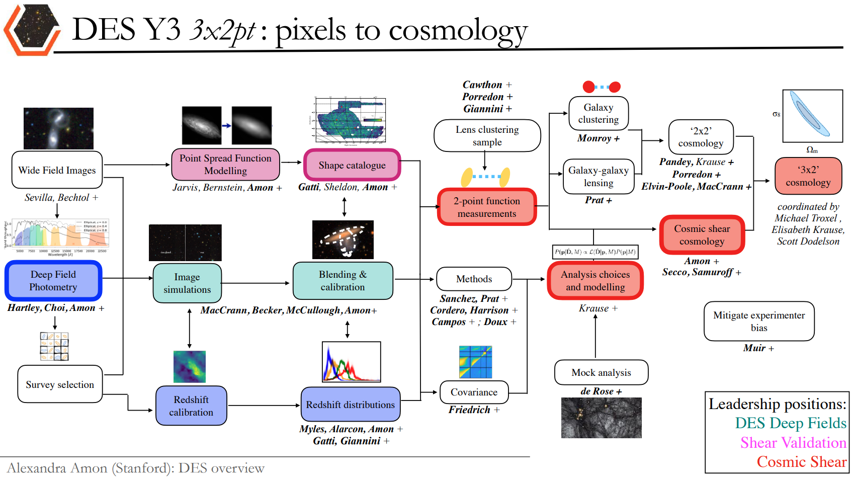
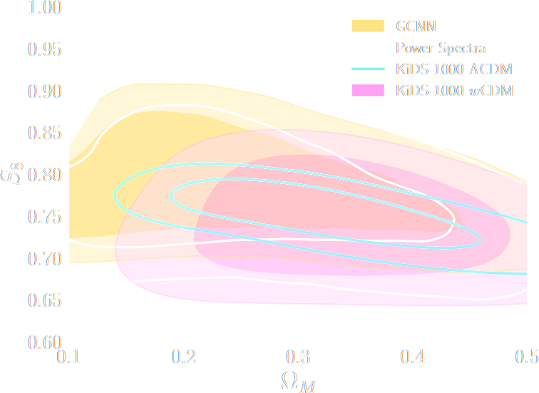
Finally, SBI has reached the mainstream: Official DES year 3 SBI wCDM results
Jeffrey et al. (2024)
I'm calling it!
Implicit Inference is solved for cosmological surveys!
@EiffL - Cagliari, June 2025
Has it delivered everything we hoped for?
Example of unforeseen impact of shortcuts in simulations
Gatti, Jeffrey, Whiteway et al. (2023)
Is it ok to distribute lensing source galaxies randomly in simulations, or should they be clustered?
$\Longrightarrow$ An SBI analysis could be biased by this effect and you would never know it!
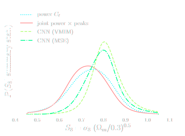
How much usable information is there beyond the power spectrum?
Chisari et al. (2018)
Ratio of power spectrum in hydrodynamical simulations vs. N-body simulations
Secco et al. (2021)
DES Y3 Cosmic Shear data vector
$\Longrightarrow$ Can we find non-Gaussian information that is not affected by baryons?
takeways
Will we be able to exploit all of the information content of
LSST, Euclid, DESI?
$\Longrightarrow$ Not rightaway, but it is not the fault of the inference
methodology!
Deep Learning has redefined the limits of our statistical
tools, creating
additional demand on the accuracy of simulations far
beyond the power spectrum.
Neural compression methods have the downside of being opaque.
It is much harder to detect unknown systematics.
We will need a significant number of
large volume, high resolution simulations.
If Implicit Inference is solved, can we still have fun solving Explicit Inference?
More seriously, Explicit Inference has some advantages:
More introspectable results to identify systematics
Allows for fitting parametric corrections/nuisances from data
Provides validation of statistical inference with a different method
Explicit Inference
Where the things are!
Simulators as Hierarchical Bayesian Models
If we have access to all latent variables $z$ of the simulator,
then the joint log likelihood $p(x | z, \theta)$ is explicit.
We need to infer the joint posterior $p(\theta, z | x)$ before marginalization to
yield $p(\theta | x) = \int p(\theta, z | x) dz$.
$\Longrightarrow$ Extremely difficult problem as $z$ is typically very high-dimensional.
Necessitates inference strategies with access to gradients of the likelihood.
$$\frac{d \log p(x | z, \theta)}{d \theta} \quad ; \quad \frac{d \log p(x | z, \theta)}{d z} $$
For instance: Maximum A Posterior estimation, Hamiltonian Monte-Carlo, Variational Inference.
$\Longrightarrow$ The only hope for explicit cosmological inference is to have fully-differentiable cosmological simulations!
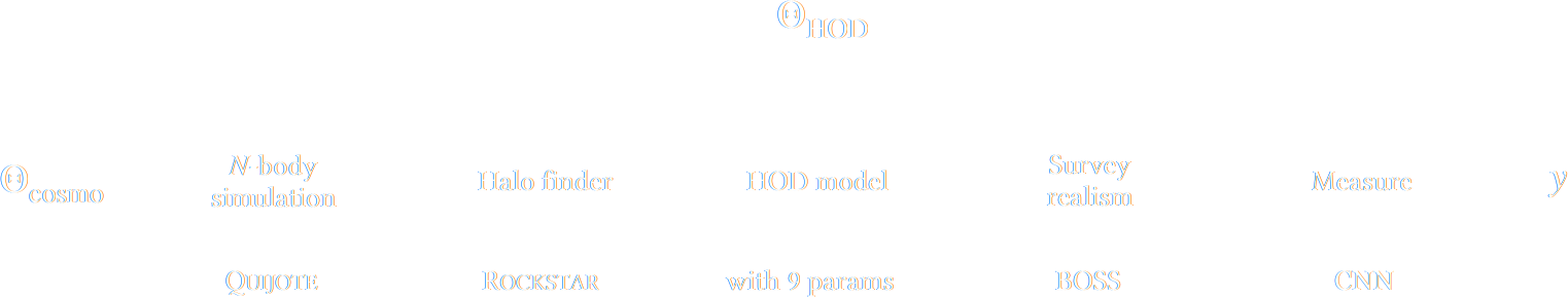
How complicated can it be to simulate the entire Universe?
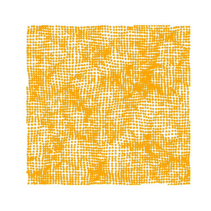
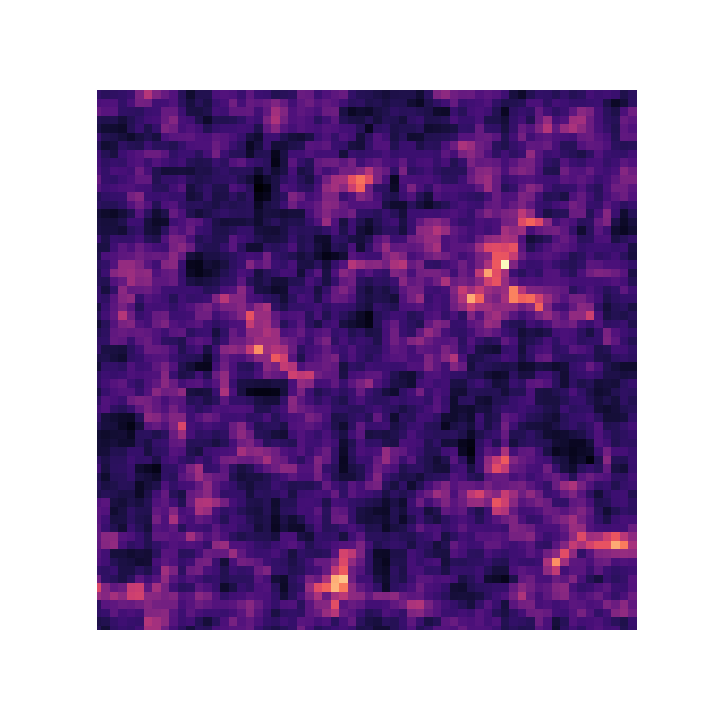
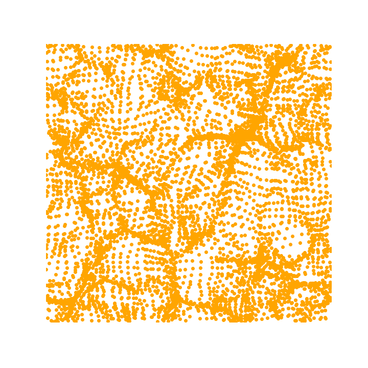
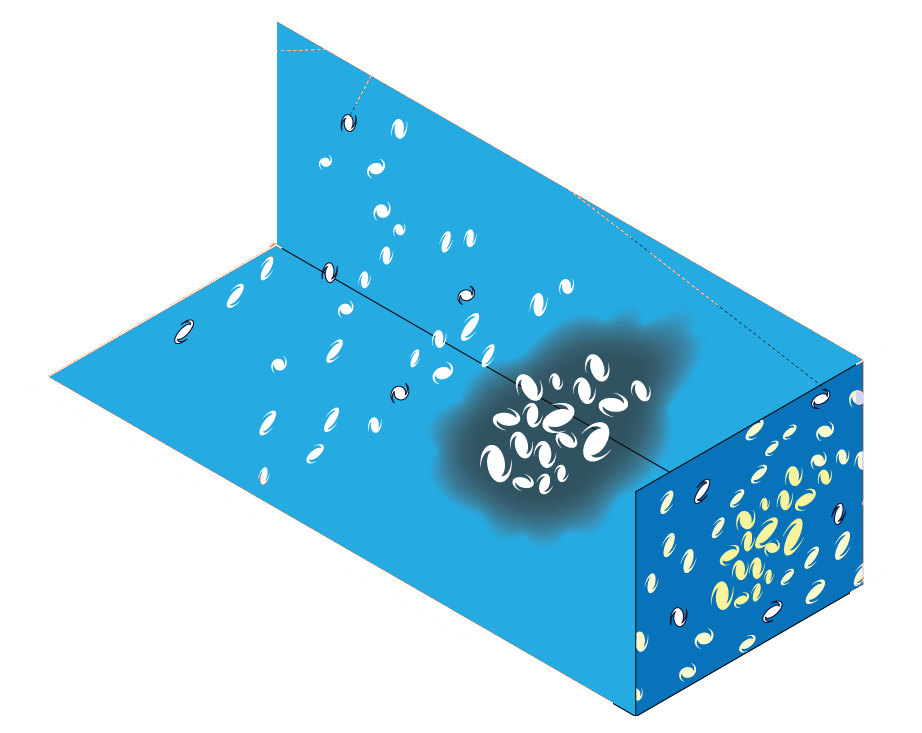
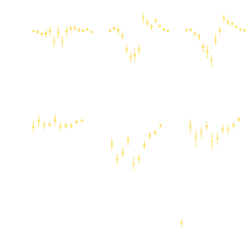
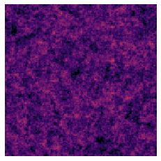
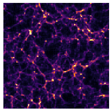
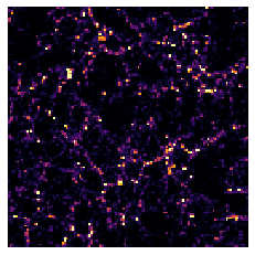
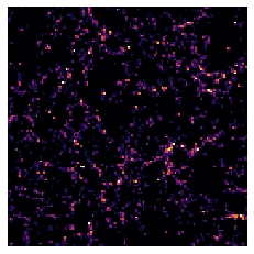
Forward Models in Cosmology
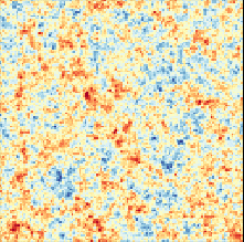
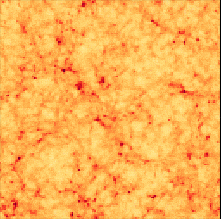
Linear Field
Final Dark Matter
Dark Matter Halos
Galaxies
$\longrightarrow$
N-body simulations
$\longrightarrow$ Group Finding algorithms
$\longrightarrow$ Semi-analytic & distribution models
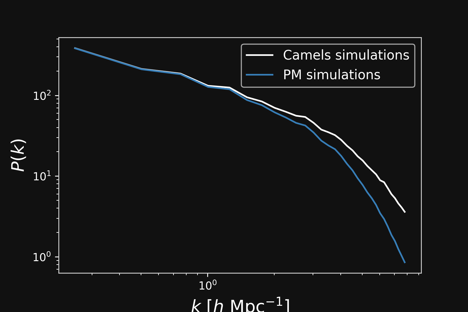
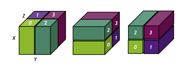
the Fast Particle-Mesh scheme for N-body simulations
The idea: approximate gravitational forces by estimating densities on a grid.
The numerical scheme:
Estimate the density of particles on a mesh
=> compute gravitational forces by FFT
Interpolate forces at particle positions
Update particle velocity and positions, and iterate
Fast and simple, at the cost of approximating short range interactions.
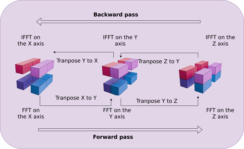
$\Longrightarrow$ Only a series of FFTs and interpolations.
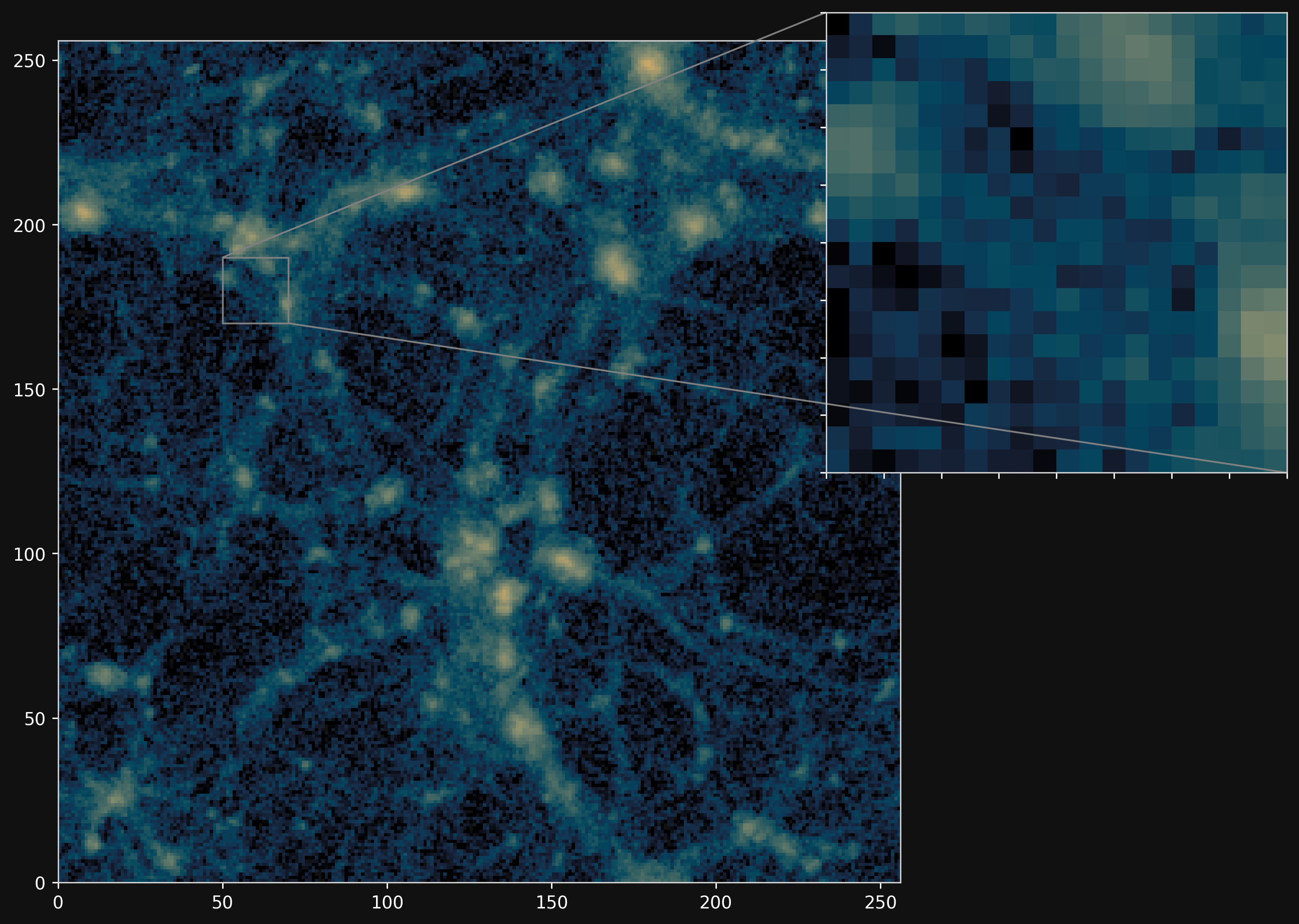
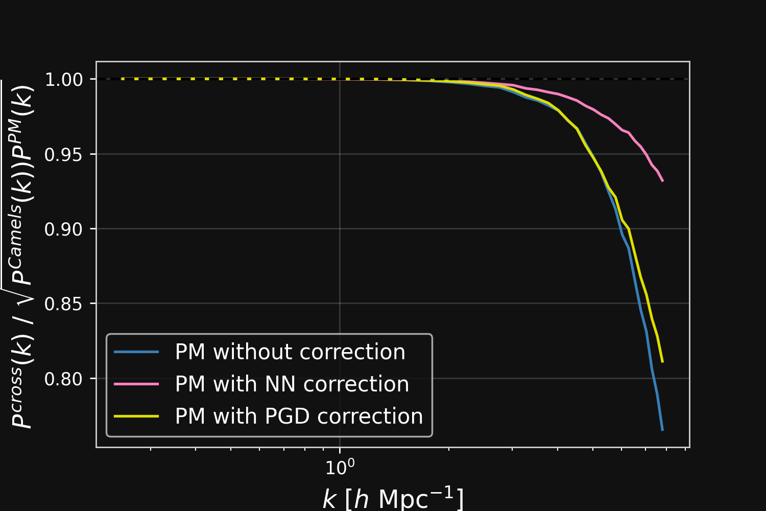
Correction integrated as a Fourier-based isotropic filter $f_{\theta}$ $\to$ incorporates translation and rotation symmetries
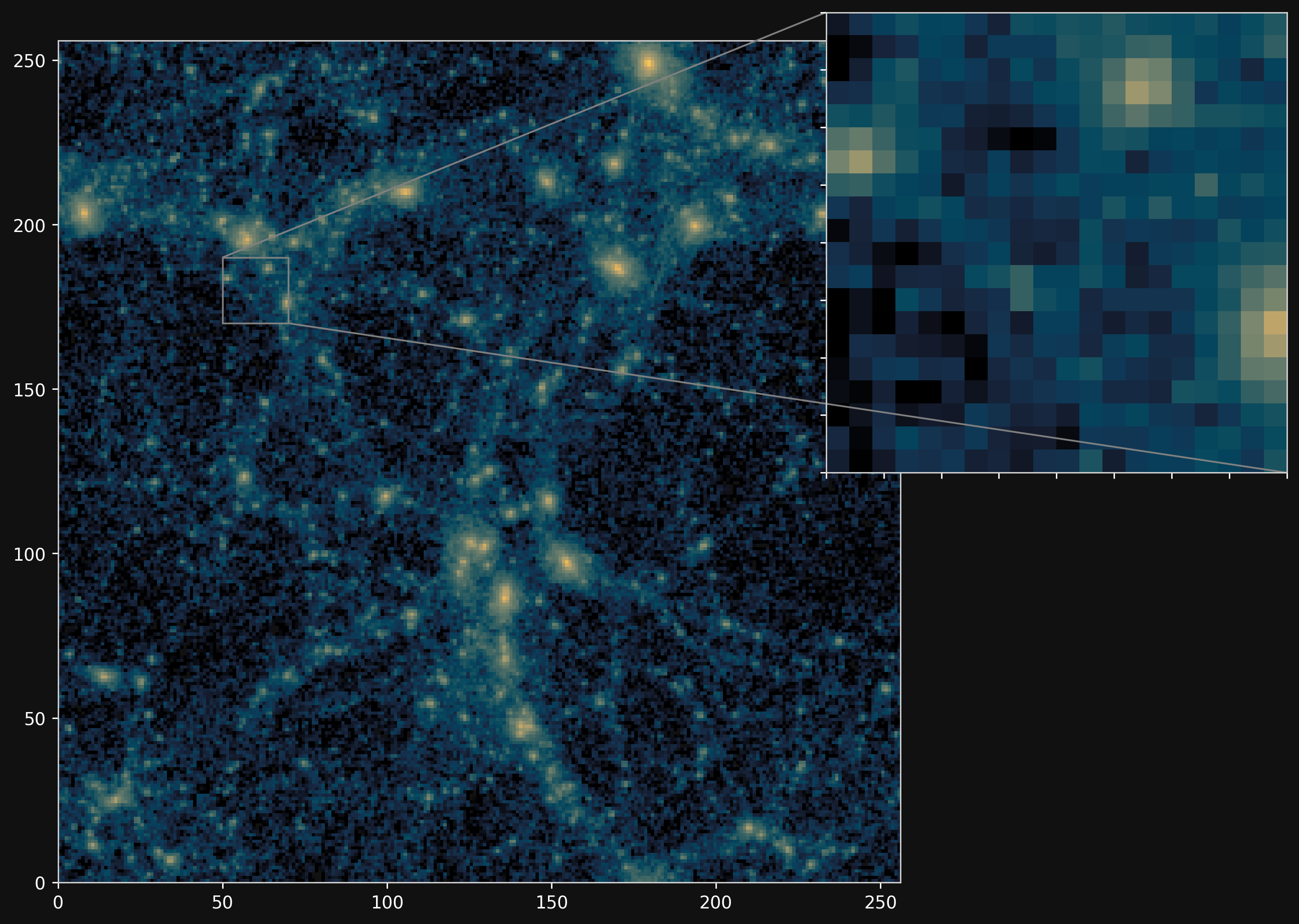
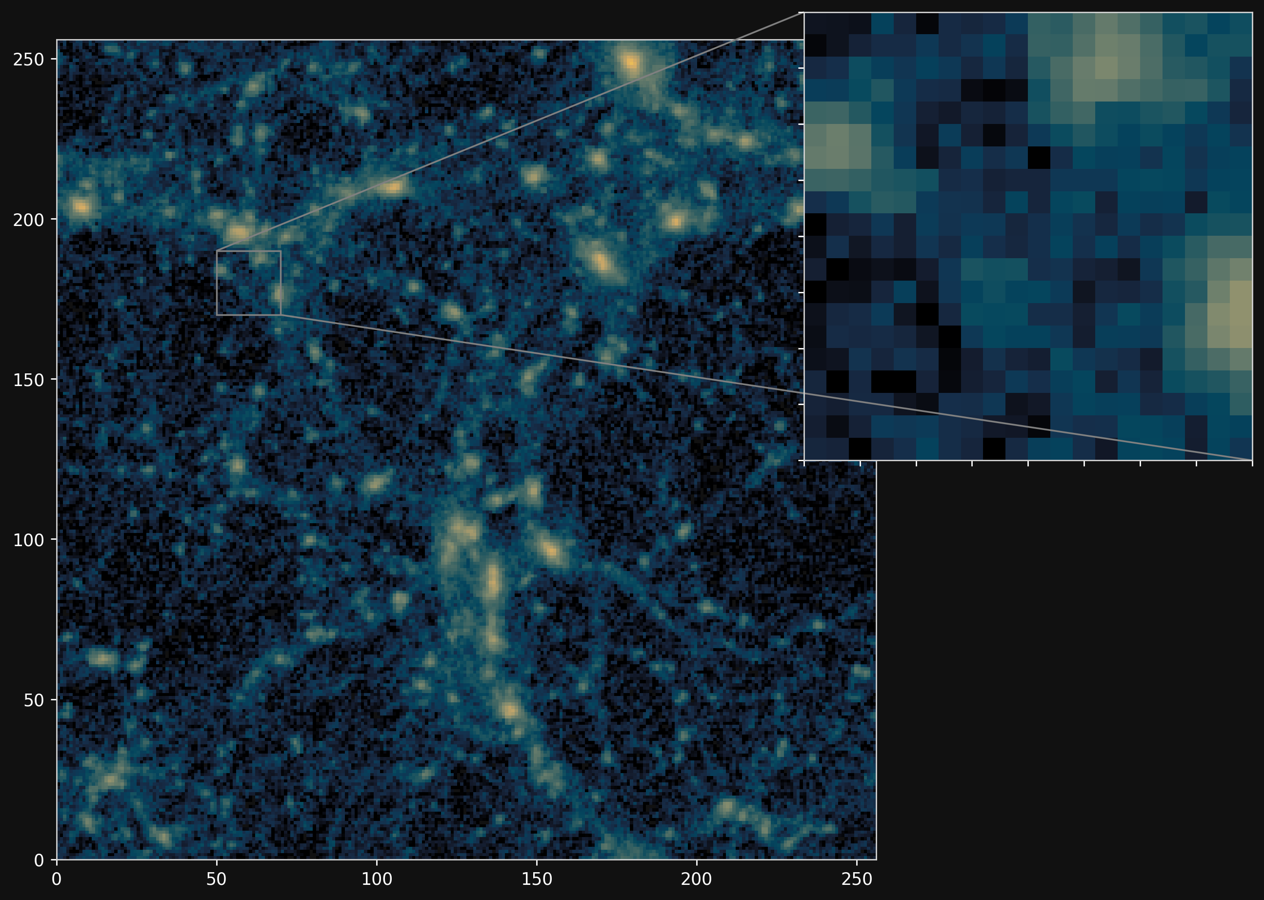
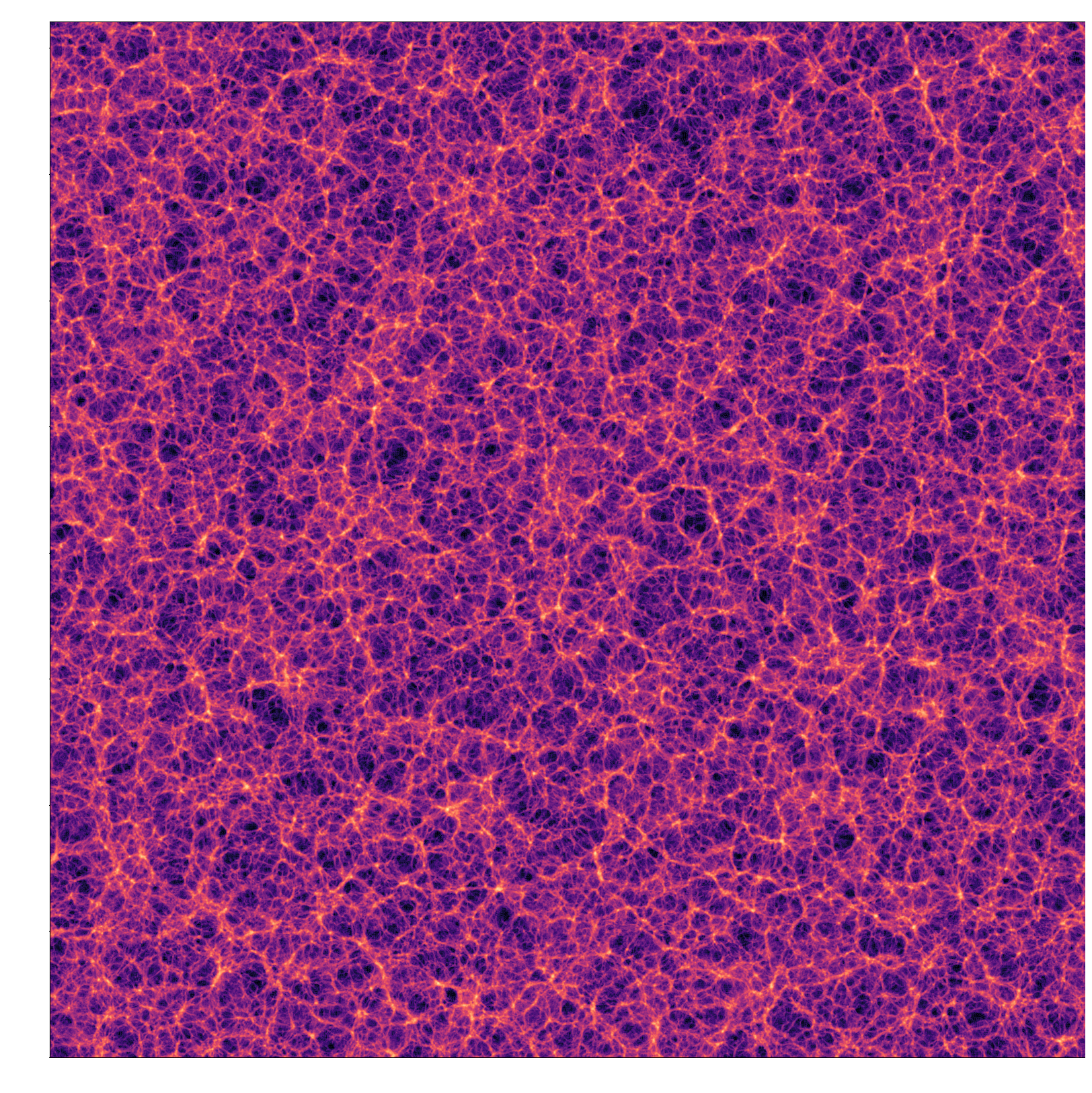
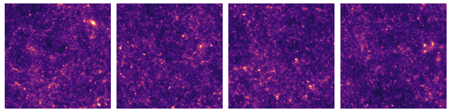
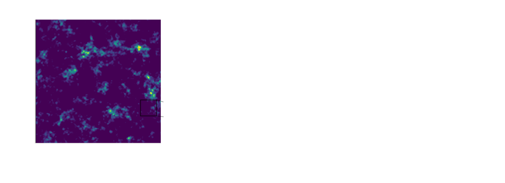
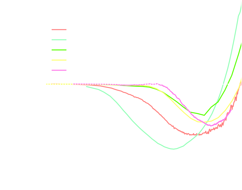
Projections of final density field
Camels simulations
PM simulations
PM+NN correction
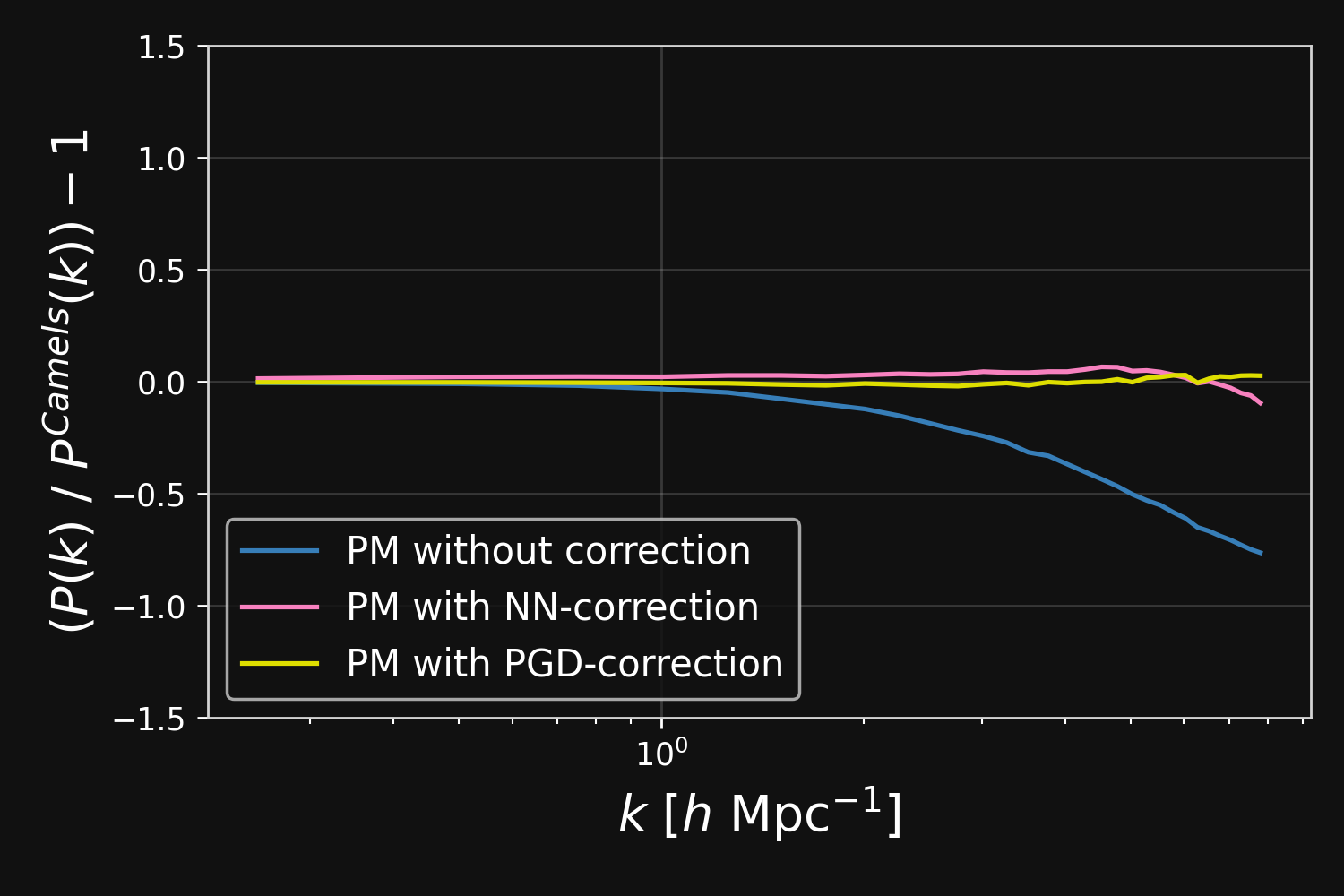
Results
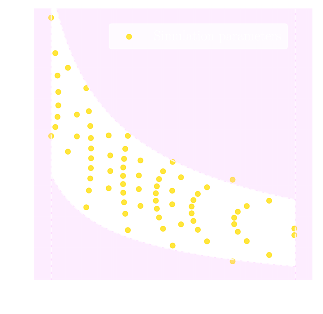
Neural network trained using single CAMELS simulation of $25^3$ ($h^{-1}$ Mpc)$^3$ volume and $64^3$ dark matter particles at the fiducial cosmology of $\Omega_m = 0.3$
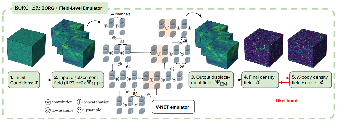
Hybrid N-body simulations with Field-Level Emulator
Jamieson et al. (2023)
Doeser et al. (2024)
Bartlett et al. (2024)
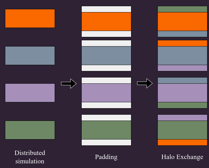
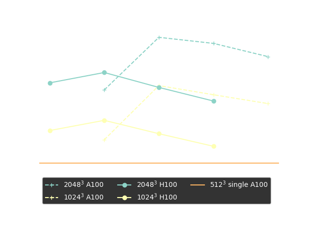
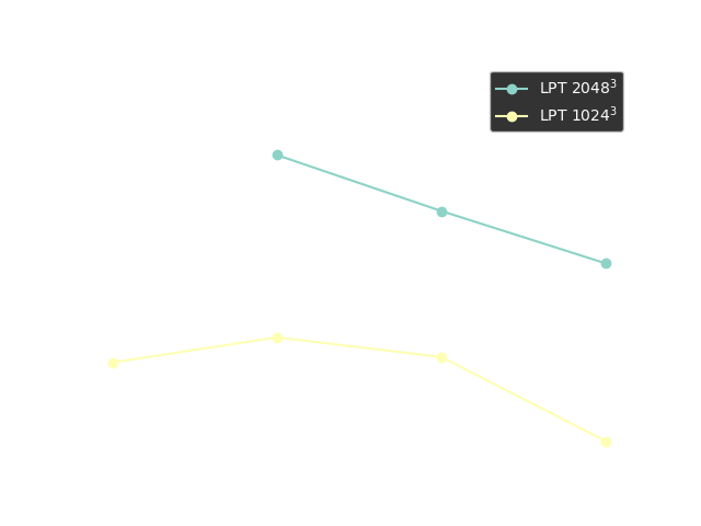
The need for distributed differentiable programming frameworks
The state vector of a moderate size cosmological simulation volume can easily require from 100GB to several TB.
$\Longrightarrow$ We need model-parallelism! Not currently fully supported by any mainstream autodiff frameworks!
(Gholami et al. 2018)
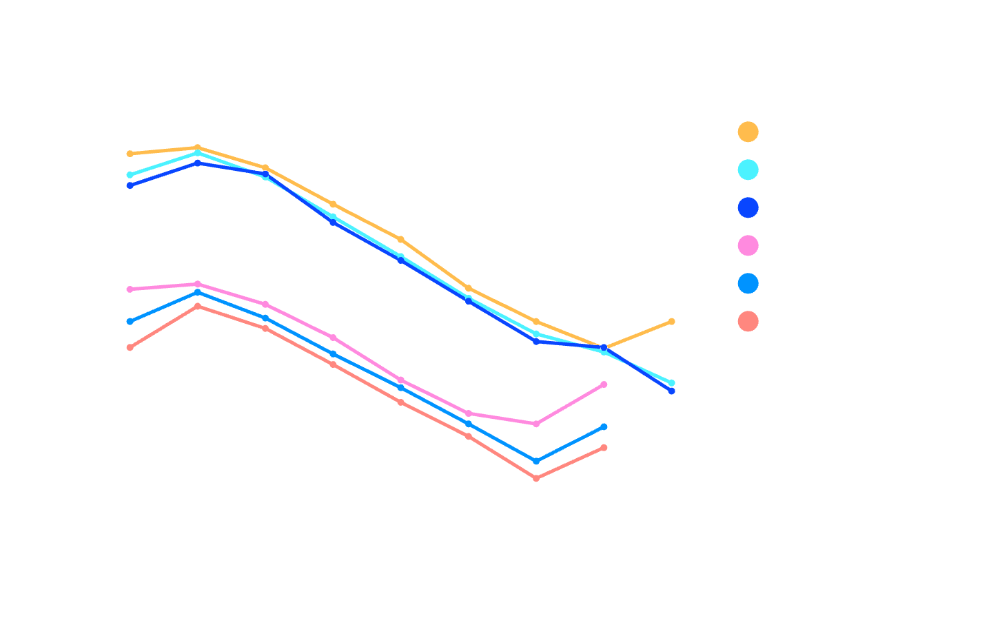
JAX-powered differentiable HPC
JAX v0.4 has made a strong push for bringing automated parallelization
and support multi-host GPU clusters!
Scientific HPC still most likely requires dedicated high-performance ops


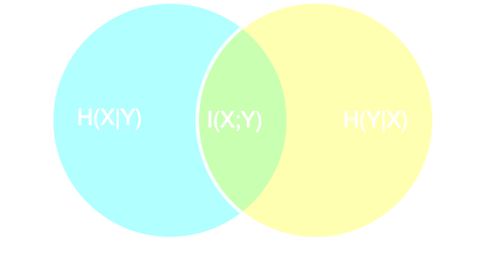

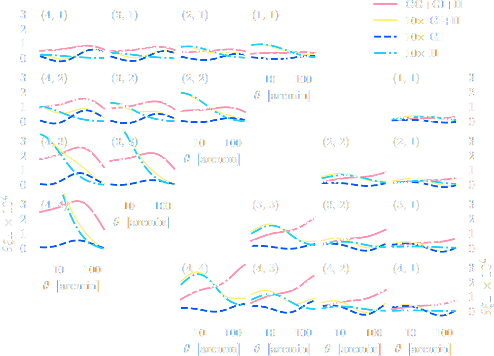
 Information Maximization Neural Network (IMNN)
$$\mathcal{L} \ = \ - | \det \mathbf{F} | \ \mbox{with} \ \mathbf{F}_{\alpha, \beta} = tr[ \mu_{\alpha}^t C^{-1} \mu_{\beta} ] $$
Information Maximization Neural Network (IMNN)
$$\mathcal{L} \ = \ - | \det \mathbf{F} | \ \mbox{with} \ \mathbf{F}_{\alpha, \beta} = tr[ \mu_{\alpha}^t C^{-1} \mu_{\beta} ] $$


 Linear Field
 Final Dark Matter
 Dark Matter Halos
 Galaxies