Introduction to Probabilistic Deep Learning
ADA X Summer School, Hersonissos, Sept. 2023
François Lanusse


Learning Objectives & Program

- Morning: Introduction to Neural Networks and Understanding Uncertainties
- What are Neural Networks and how to code them
- Combining Neural Networks and Probabilities to perform Bayesian Inference
- Afternoon: Deep Generative Modeling and Application to Inverse Problems
- How to solve inverse problems from a Bayesian point of view
- How to model high dimensional distributions with Deep Generative Models
- Building your own Normalizing Flow in JAX/Flax/Tensorflow Probability
- Deconvolving Galaxy Images from the HSC survey with Deep Generative Priors
A (very) Brief Introduction to Neural Architectures
What is a neural network?
Simplest architecture: Multilayer Perceptron (MLP)
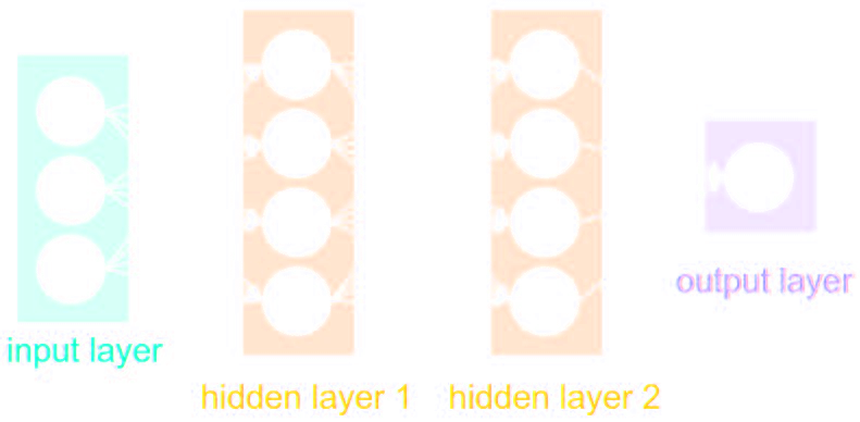
- Series of Dense a.k.a Fully connected layers:
$$ h = \sigma(W x + b)$$
where:
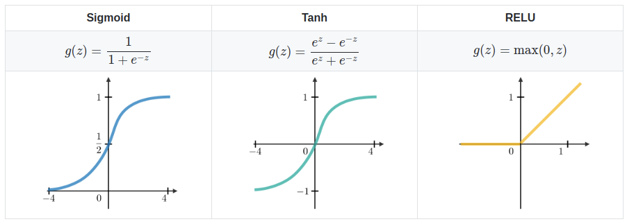
- $\sigma$ is the activation function (e.g. ReLU, Sigmoid, etc.)
- $W$ is a multiplicative weight matrix
- $b$ is an additive bias parameter
- This defines a parametric non-linear function $f_\theta(x)$
- MLPs are universal function approximators
Nota bene: only asymptotically true!
How do you use it to approximate functions?
- Assume a loss function that should be small for good approximations on a training set of data points $(x_i, y_i)$ $$ \mathcal{L} = \sum_{i} ( y_i - f_\theta(x_i))^2 $$
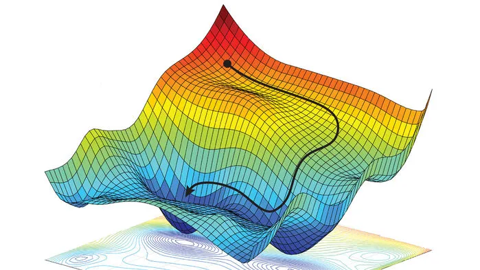
- Optimize the parameters $\theta$ to minimize the loss function by gradient descent $$ \theta_{t+1} = \theta_t - \eta \nabla_\theta \mathcal{L} $$
Different neural architectures for different types of data
Performance can be improved for particular types of data by making use of inductive biases
 $$ h = \sigma(W \ast x + b)$$

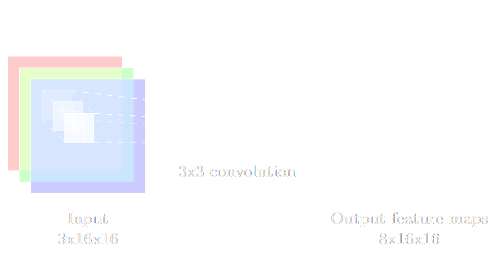
- Image -> Convolutional Networks
- Convolutional layers are translation invariant
- Pixel topology is incorporated by construction
- Time Series -> Recurrent Networks
- Temporal information and variable length is incorporated by construction
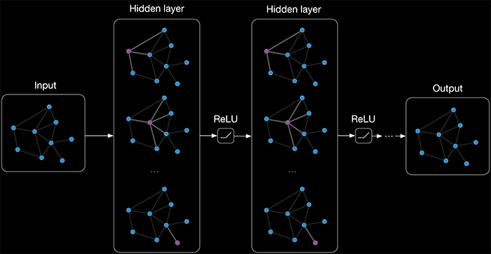
- Graph-stuctured data -> Graph Neural Networks
- Graph topology is incorporated by construction
- Can be seen as generalisation of convolutional networks
takeways
- Depending on the data, different architectures will benefit from different inductive biases.
- In 2023, you can assume that there exists a
neural architecture that can achieve near optimal performance on your data.
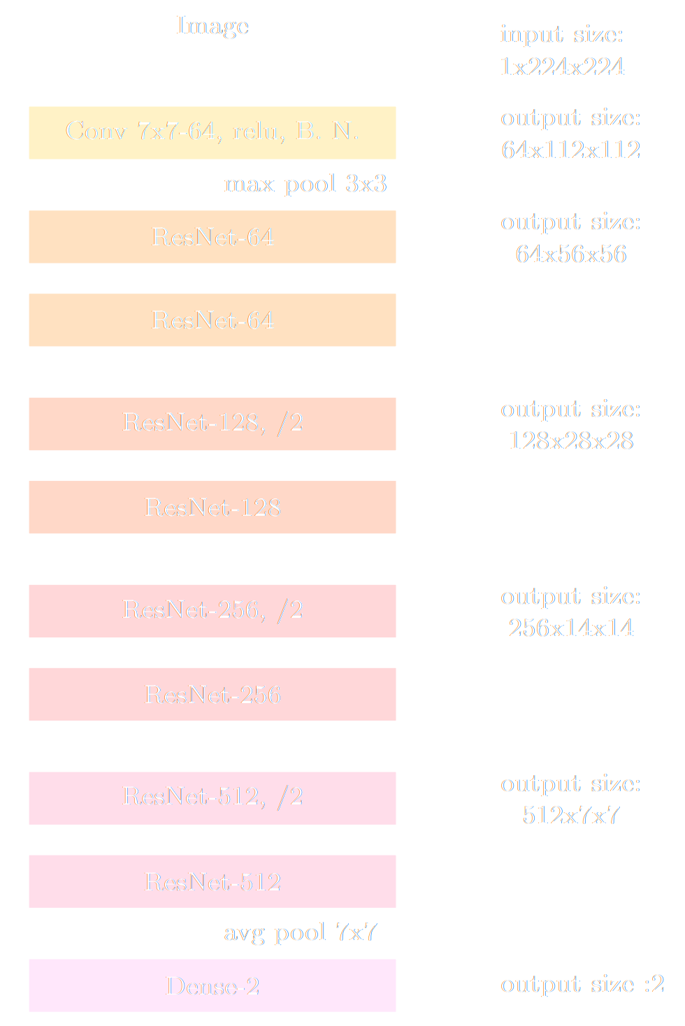
Pro tips:- Don't try to reinvent your own architecture, use an existing state of the art one! (e.g. ResNet)
- Most neural network libraries already have most common architectures implemented for you
- The particular neural network you use becomes an implementation detail.
$\Longrightarrow$ In the rest of this talk most neural networks will just be denoted by a parametric function $f_\theta$
Let's move on to the practice!
Our case study: Dynamical Mass Measurement for Galaxy Clusters
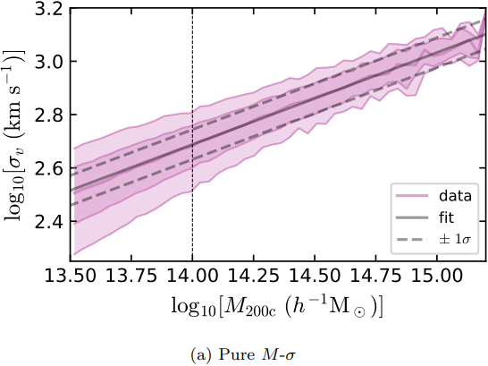
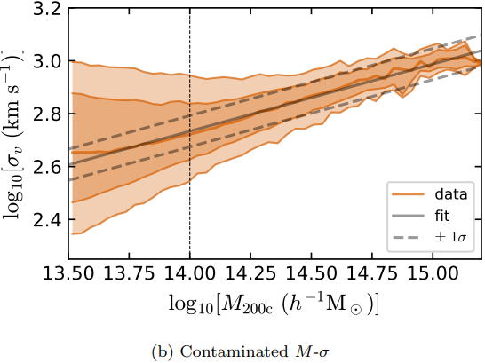
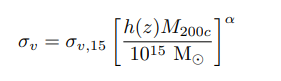
Our goal: train a neural network to estimate the cluster mass
What we will feed the model:
- Richness
- Velocity Dispersion
- Information about member galaxies:
- radial distribution
- stellar mass distribution
- LOS velocity distribution
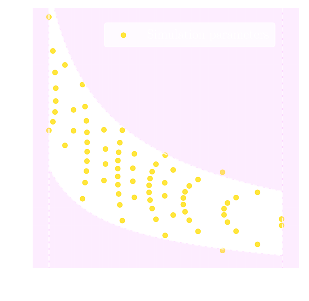
Training data from MultiDark Planck 2 N-body simulation (Klypin et al. 2016) with 261287 clusters.
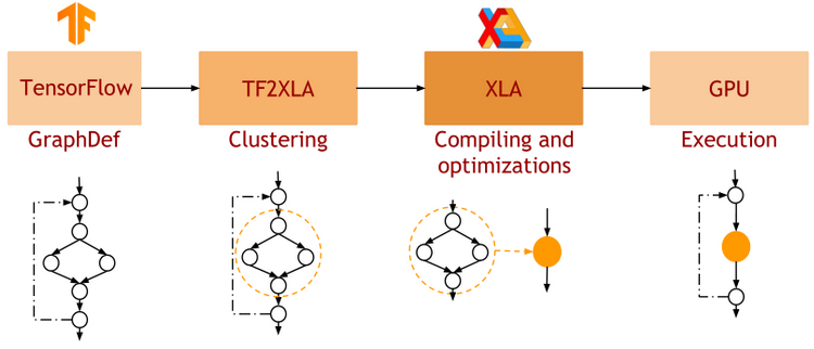
Why JAX?
and what is it?

JAX: NumPy + Autograd + XLA
- JAX uses the NumPy API
=> You can copy/paste existing code, works pretty much out of the box
- JAX is a successor of autograd
=> You can transform any function to get forward or backward automatic derivatives (grad, jacobians, hessians, etc)
- JAX uses XLA as a backend
=> Same framework as used by TensorFlow (supports CPU, GPU, TPU execution)
import jax.numpy as np

m = np.eye(10) # Some matrix

def my_func(x):
	return m.dot(x).sum()

x = np.linspace(0,1,10)
y = my_func(x)
from jax import grad

df_dx = grad(my_func)
y = df_dx(x)
Writing a Neural Network in JAX/Flax
import flax.linen as nn
import optax

class MLP(nn.Module):
	@nn.compact
	def __call__(self, x):
	x = nn.relu(nn.Dense(128)(x))
	x = nn.relu(nn.Dense(128)(x))
	x = nn.Dense(1)(x)
	return x
# Instantiate the Neural Network
model = MLP()
# Initialize the parameters
params = model.init(jax.random.PRNGKey(0), x)
prediction = model.apply(params, x)
# Instantiate Optimizer
tx = optax.adam(learning_rate=0.001)
opt_state = tx.init(params)
# Define loss function
def loss_fn(params, x, y):
	mse = model.apply(params, x) -y)**2
	return jnp.mean(mse)
# Compute gradients
grads = jax.grad(loss_fn)(params, x, y)
# Update parameters
updates, opt_state = tx.update(grads, opt_state)
params = optax.apply_updates(params, updates)

- Model Definition: Subclass the flax.linen.Module base class. Only need to define the __call__() method.
-
Using the Model: the model instance provides 2 important methods:
- init(seed, x): Returns initial parameters of the NN
- apply(params, x): Pure function to apply the NN
- Training the Model: Use jax.grad to compute gradients and Optax optimizers to update parameters
Now you try it!
We will be using this notebook: https://bit.ly/3LaLHq3Your goal: Building a regression model with a Mean Squared Error loss in JAX/Flax
def loss_fn(params, x, y):
  mse = (model.apply(params, x) - y)**2
  return jnp.mean(mse)
Raise your hand if you manage to get a cluster mass prediction!
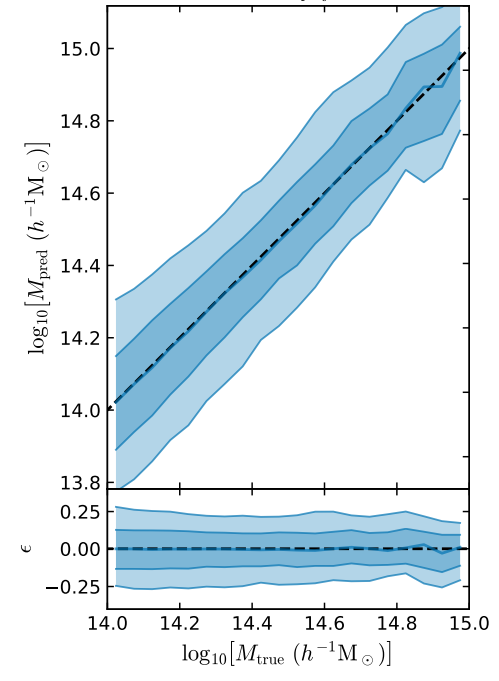
First attempt with an MSE loss
class MLP(nn.Module):
@nn.compact
def __call__(self, x):
	x = nn.relu(nn.Dense(128)(x))
	x = nn.relu(nn.Dense(128)(x))
	x = nn.tanh(nn.Dense(64)(x))
	x = nn.Dense(1)(x)
	return x

def loss_fn(params, x, y):
	prediction = model.apply(params, x)
return jnp.mean( (prediction - y)**2 )- The prediction appears to be biased... What is going on?
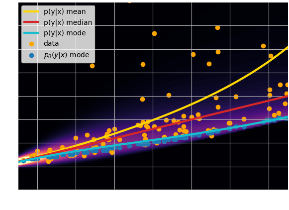
A neural network will try to answer
the question you ask.
Let's try to understand the neural network output by looking at the loss function
$$ \mathcal{L} = \sum_{(x_i, y_i) \in \mathcal{D}} \parallel x_i - f_\theta(y_i)\parallel^2 \quad \simeq \quad \int \parallel x - f_\theta(y) \parallel^2 \ p(x,y) \ dx dy $$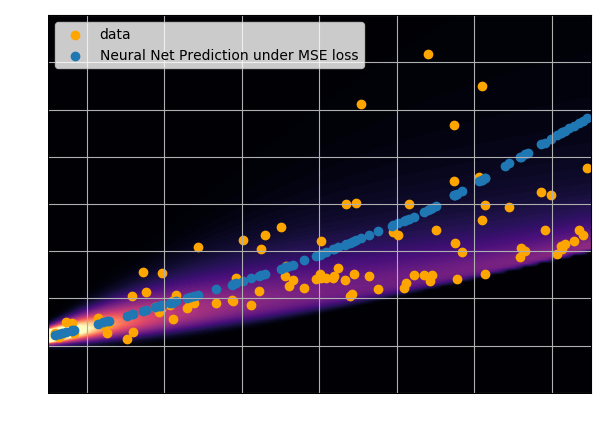
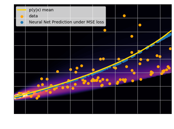
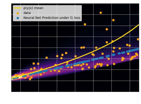
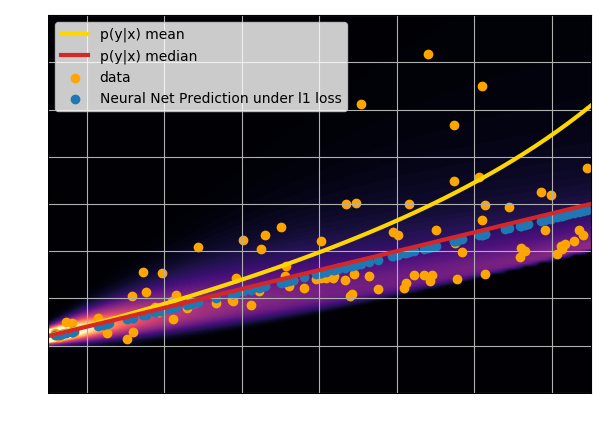
- Using an $\ell_2$ loss learns the mean of the $p(x | y)$
- Using an $\ell_1$ loss learns the median of $p(x|y)$
- In general, training a neural network for
regression doesn't
achieve de mode of the distribution.
Check this blogpost and this notebook to learn how to do that:
Let's take a step back and think as Bayesians
In our case here:
- The prior $p(x)$ would be an assumption on plausible cluster masses
- The likelihood $p(y |x)$ is the probability of observing particular cluster poperties for clusters of a given mass
- Where do my priors and likelihoods come from in this case?
- How do I ask a neural network to solve the full Bayesian inference problem?
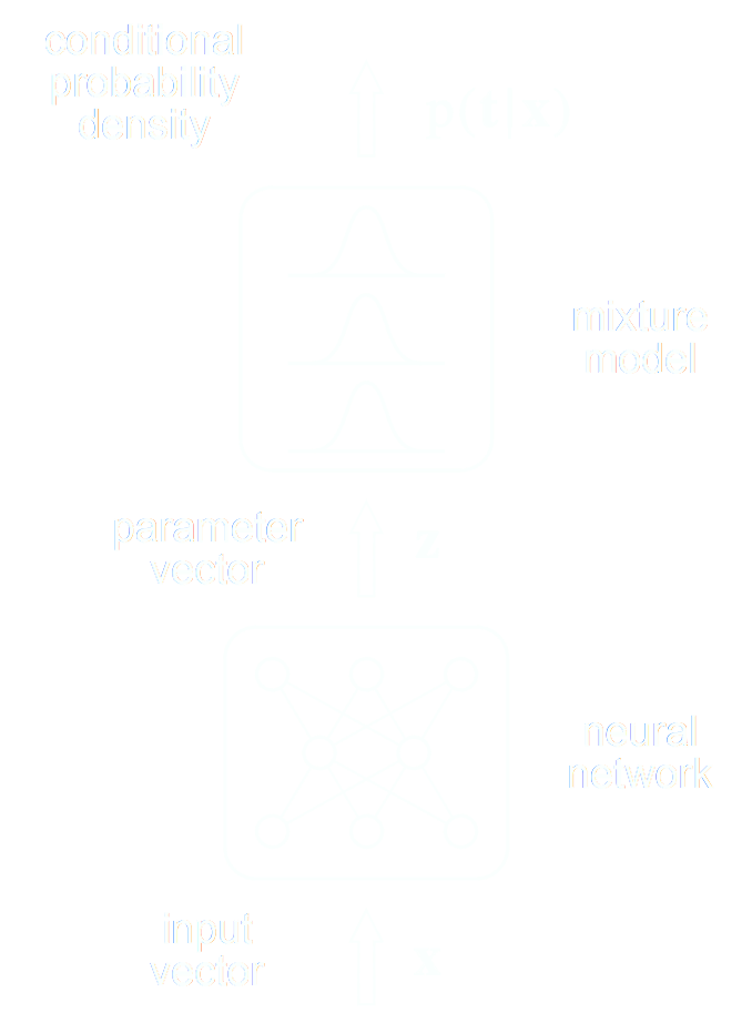
- Mixture Density Networks (MDN) \begin{equation} q_\phi(x | y) = \prod_i \pi^i_\phi(y) \ \mathcal{N}\left(\mu^i_\phi(y), \ \sigma^i_\phi(y) \right) \nonumber \end{equation}
- Flourishing Machine Learning literature on density estimators for higher dimensions. (more on this this afternoon)
![]() GLOW, (Kingma & Dhariwal, 2018)
GLOW, (Kingma & Dhariwal, 2018)

 The Kullback-Leibler divergence:
$$ D_{KL}(p||q) = \mathbb{E}_{x \sim p(x)} \left[ \log \frac{p(x)}{q(x)} \right] $$
The Kullback-Leibler divergence:
$$ D_{KL}(p||q) = \mathbb{E}_{x \sim p(x)} \left[ \log \frac{p(x)}{q(x)} \right] $$
Sampling from the joint distribution can be expressed as: $$ (x, y) \sim p(x, y) = \underbrace{p(y | x)}_{\mathrm{likelihood}} \ \underbrace{p(x)}_{\mathrm{prior}} $$
- Priors AND likelihoods are hardcoded in the training set.
- If your data is based on simulations you control both
- If your data is observational, be very careful and cognizant of the fact that selection effects in your dataset translate as implicit priors.
Summarizing the Probabilistic Deep Learning Recipe
- Express the output of the model as a distribution, not a point estimate $$ q_\phi(x | y) $$
- Assemble a training set that encodes your prior on the problem $$ \mathcal{D} = \left\{ (x_i, y_i) \sim p(x, y) = p(y|x) p(x) \right\} $$
- Optimize for the Negative Log Likelihood $$\mathcal{L} = - \log q_\phi(x|y) $$
- Profit!
- Interpretable network outputs (i.e. I know mathematically what my network is trying to approximate)
- Uncertainty quantification (i.e. Bayesian Inference)
We will need a new tool to go probabilistic!
TensorFlow Probability
import jax
import jax.numpy as jnp
from tensorflow_probability.substrates import jax as tfp
tfd = tfp.distributions

### Create a mixture of two scalar Gaussians:
gm = tfd.MixtureSameFamily(
	mixture_distribution=tfd.Categorical(
					probs=[0.3, 0.7]),
	components_distribution=tfd.Normal(
					loc=[-1., 1],
					scale=[0.1, 0.5]))

# Evaluate probability
gm.log_prob(1.0)
Let's build a Conditional Density Estimator in JAX/Flax/TFP
class MDN(nn.Module):
	num_components: int

	@nn.compact
	def __call__(self, x):
		x = nn.relu(nn.Dense(128)(x))
		x = nn.relu(nn.Dense(128)(x))
		x = nn.tanh(nn.Dense(64)(x))

		# Instead of regressing directly the value of the mass, the network
		# will now try to estimate the parameters of a mass distribution.
		categorical_logits = nn.Dense(self.num_components)(x)
		loc = nn.Dense(self.num_components)(x)
		scale = 1e-3 + nn.softplus(nn.Dense(self.num_components)(x))

		dist =tfd.MixtureSameFamily(
			mixture_distribution=tfd.Categorical(logits=categorical_logits),
			components_distribution=tfd.Normal(loc=loc, scale=scale))

		# To make it understand the batch dimension
		dist =  tfd.Independent(dist)

		# Returns a distribution !
		return dist
Now you try it!
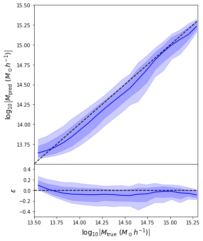
Let's go back to our notebookYour next goal: Implement a Mixture Density Network in JAX/Flax/TFP, and use it to get an unbiased mass estimate.
def loss_fn(params, x, y):
	q = model.apply(params, x)
	return jnp.mean( - q.log_prob(y[:,0]) )
Raise your hand if you manage to get a cluster mass prediction with this new model!
takeaways
- Unless the relationship between input and outputs of your problem is purely deterministic (e.g. power spectrum emulator), you should think under a probabilistic model to understand what the network is doing.
- Conditional density estimation is superior to point estimates
- Provides uncertainty quantification
- Even if a point estimate is desired, gives access to the Maximum a Posteriori
- We have learned how to pose a Deep Learning question:
- A loss function $\mathcal{L}$ and training set $\mathcal{D}$
$\Longrightarrow$ Mathematically defines the solution you are trying to get. - An appropriate architecture $q_\phi$
$\Longrightarrow$ This is the tool you are using to solve the problem.
- A loss function $\mathcal{L}$ and training set $\mathcal{D}$
Example of Application:
Simulation-Based Inference
The limits of traditional cosmological inference
- Measure the ellipticity $\epsilon = \epsilon_i + \gamma$ of all galaxies
$\Longrightarrow$ Noisy tracer of the weak lensing shear $\gamma$ - Compute summary statistics based on 2pt functions,
e.g. the power spectrum - Run an MCMC to recover a posterior on model parameters, using an analytic likelihood $$ p(\theta | x ) \propto \underbrace{p(x | \theta)}_{\mathrm{likelihood}} \ \underbrace{p(\theta)}_{\mathrm{prior}}$$
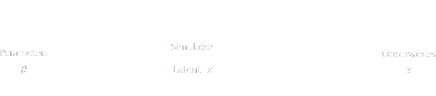
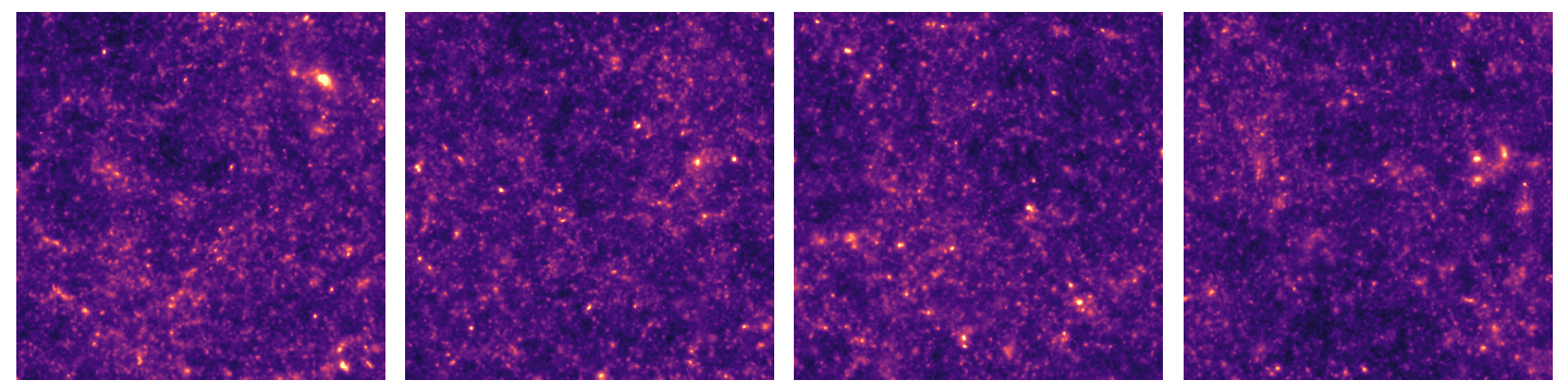
Full-Field Simulation-Based Inference
- Instead of trying to analytically evaluate the likelihood of
sub-optimal summary statistics, let us build a forward model of the full observables.
$\Longrightarrow$ The simulator becomes the physical model. - Each component of the model is now tractable, but at the cost of a large number of latent variables.
- Fully exploits the information content of the data (aka "full field inference").
- Easy to incorporate systematic effects.
- Easy to combine multiple cosmological probes by joint simulations.
...so why is this not mainstream?
$\Longrightarrow$ This marginal likelihood is intractable!
Black-box Simulators Define Implicit Distributions
- A black-box simulator defines $p(x | \theta)$ as an implicit distribution, you can sample from it but you cannot evaluate it.
- Key Idea: Use a parametric distribution model $\mathbb{P}_\varphi$ to approximate the implicit distribution $\mathbb{P}$.

True $\mathbb{P}$

Samples $x_i \sim \mathbb{P}$

Model $\mathbb{P}_\varphi$
Deep Learning Approaches to Implicit Inference
- Automatically learn an optimal low-dimensional summary statistic $$y = f_\varphi(x) $$
- Use Neural Density Estimation to either:
- build an estimate $p_\phi$ of the likelihood function $p(y \ | \ \theta)$ (Neural Likelihood Estimation)
- build an estimate $p_\phi$ of the posterior distribution $p(\theta \ | \ y)$ (Neural Posterior Estimation)
Automated Summary Statistics Extraction
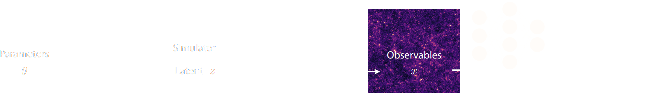
- Introduce a parametric function $f_\varphi$ to reduce the dimensionality of the data while preserving information.
- Summary statistics $y$ is sufficient for $\theta$ if $$ I(Y; \Theta) = I(X; \Theta) \Leftrightarrow p(\theta | x ) = p(\theta | y) $$
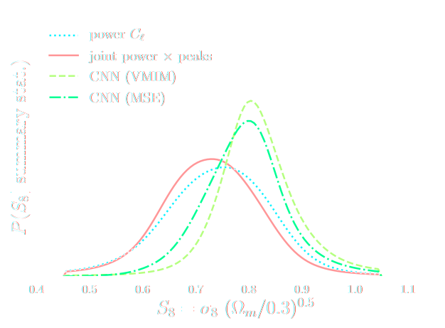
- Variational Mutual Information Maximization
$$ \mathcal{L} \ = \ \mathbb{E}_{x, \theta} [ \log q_\phi(\theta | f_\varphi(x)) ] \leq I(Y; \Theta) $$
Jeffrey, Alsing, Lanusse (2021)

Unrolling the Probabilistic Learning Recipe
- I assume a forward model of the observations: \begin{equation} p( x ) = p(x | \theta) \ p(\theta) \nonumber \end{equation} All I ask is the ability to sample from the model, to obtain $\mathcal{D} = \{x_i, \theta_i \}_{i\in \mathbb{N}}$
- I am going to assume $q_\phi(\theta | x)$ a parametric conditional density
- Optimize the parameters $\phi$ of $q_{\phi}$ according to \begin{equation} \min\limits_{\phi} \sum\limits_{i} - \log q_{\phi}(\theta_i | x_i) \nonumber \end{equation} In the limit of large number of samples and sufficient flexibility \begin{equation} \boxed{q_{\phi^\ast}(\theta | x) \approx p(\theta | x)} \nonumber \end{equation}
the Bayesian joint distribution
a simulated training set.
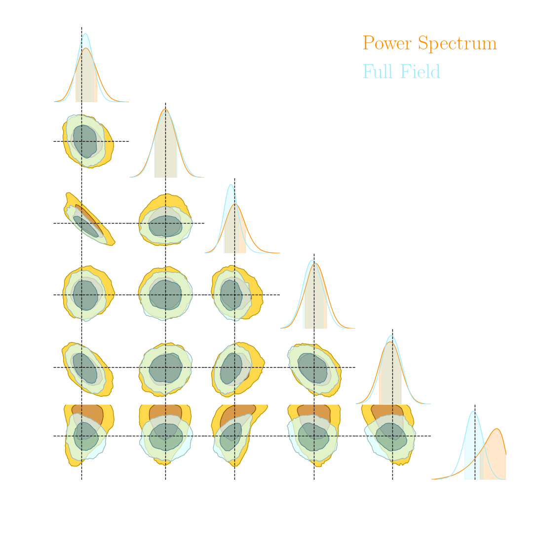
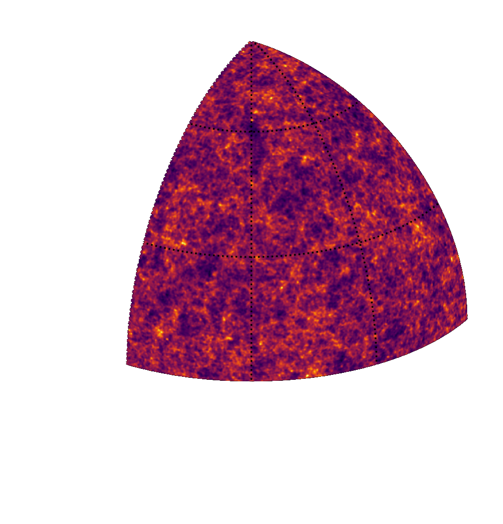
Illustration on log-normal lensing simulations

DifferentiableUniverseInitiative/sbi_lens
JAX-based log-normal lensing simulation package
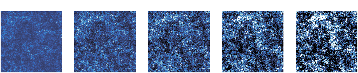
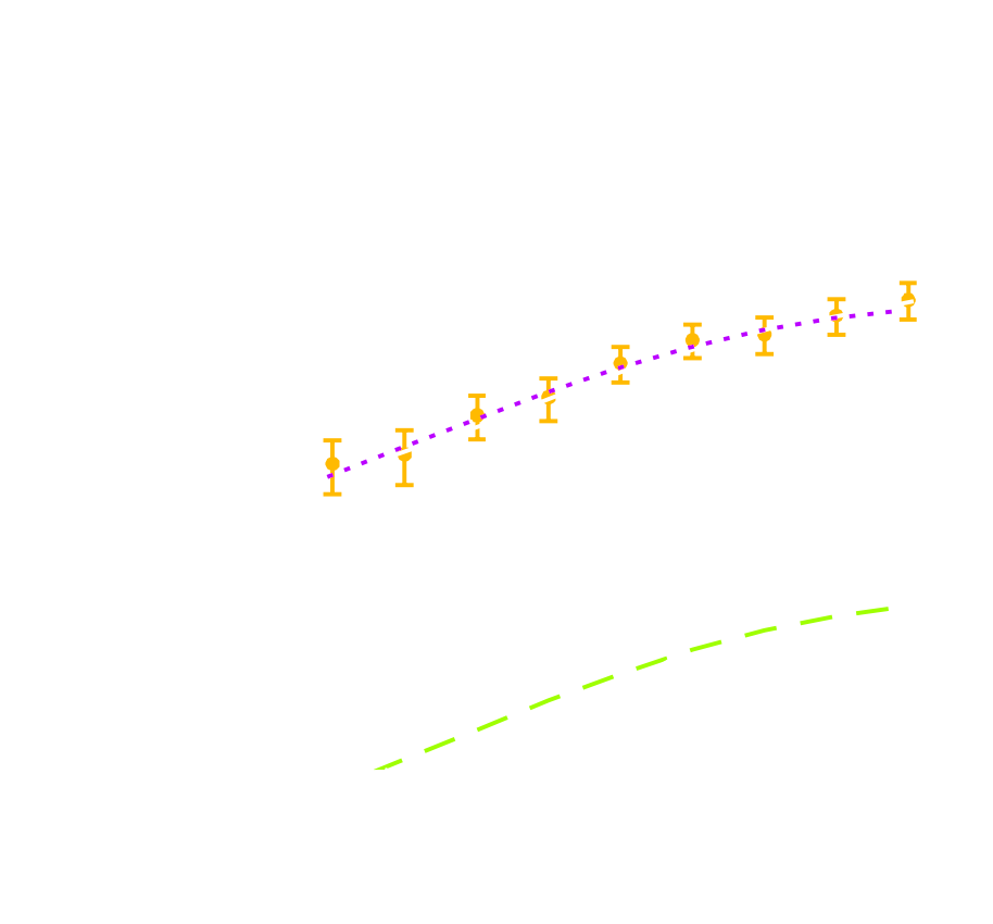
- 10x10 deg$^2$ maps at LSST Y10 quality, conditioning the log-normal shift parameter on $(\Omega_m, \sigma_8, w_0)$
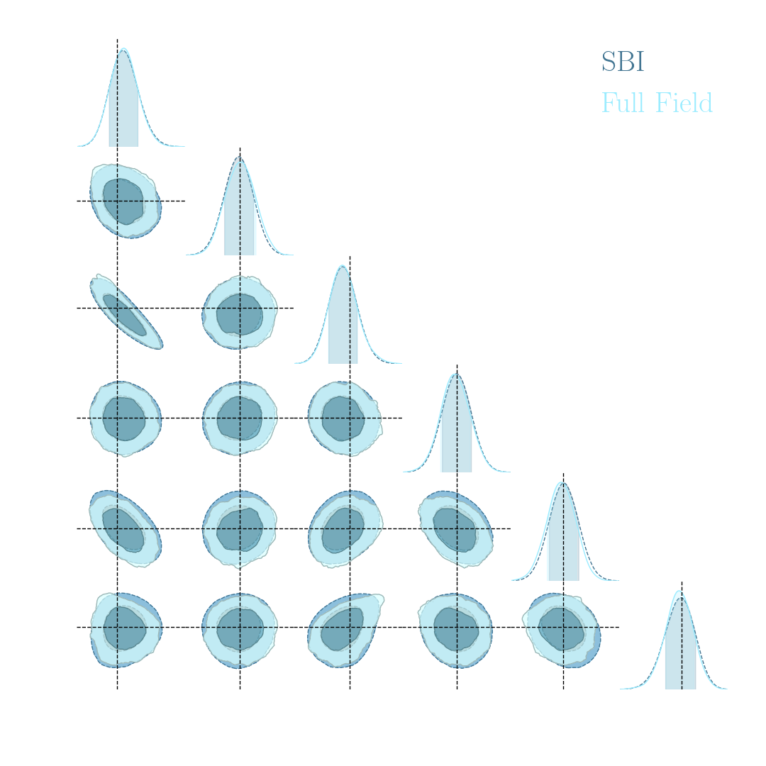
- Infer full-field posterior on cosmology:
- explicitly using an Hamiltonian-Monte Carlo (NUTS) sampler
- implicitly using a learned summary statistics and conditional density estimation.
A variety of algorithms
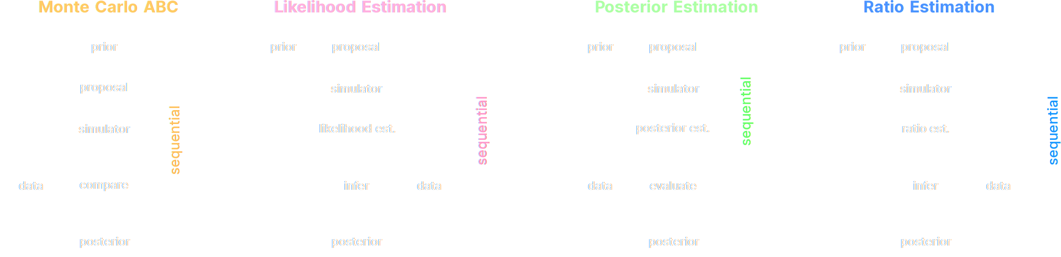
A few important points:
- Amortized inference methods, which estimate $p(\theta | x)$, can greatly speed up posterior estimation once trained.
- Sequential Neural Posterior/Likelihood Estimation methods can actively sample simulations needed to refine the inference.
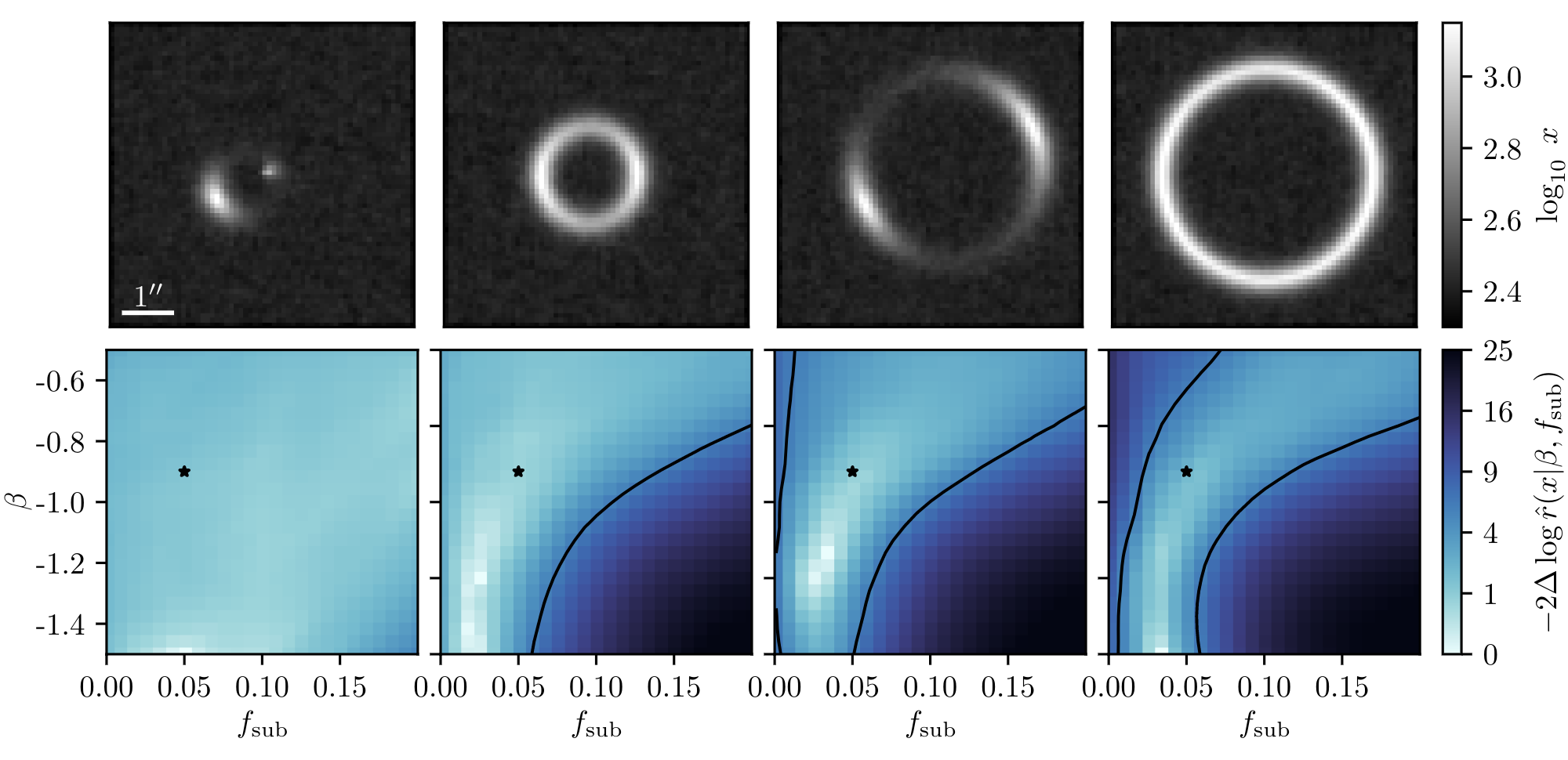
Example of application: Constraining Dark Matter Substructures

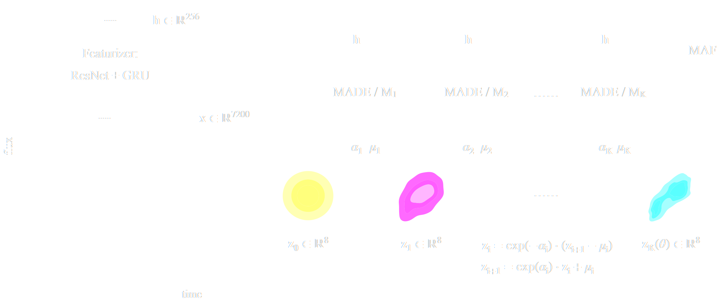
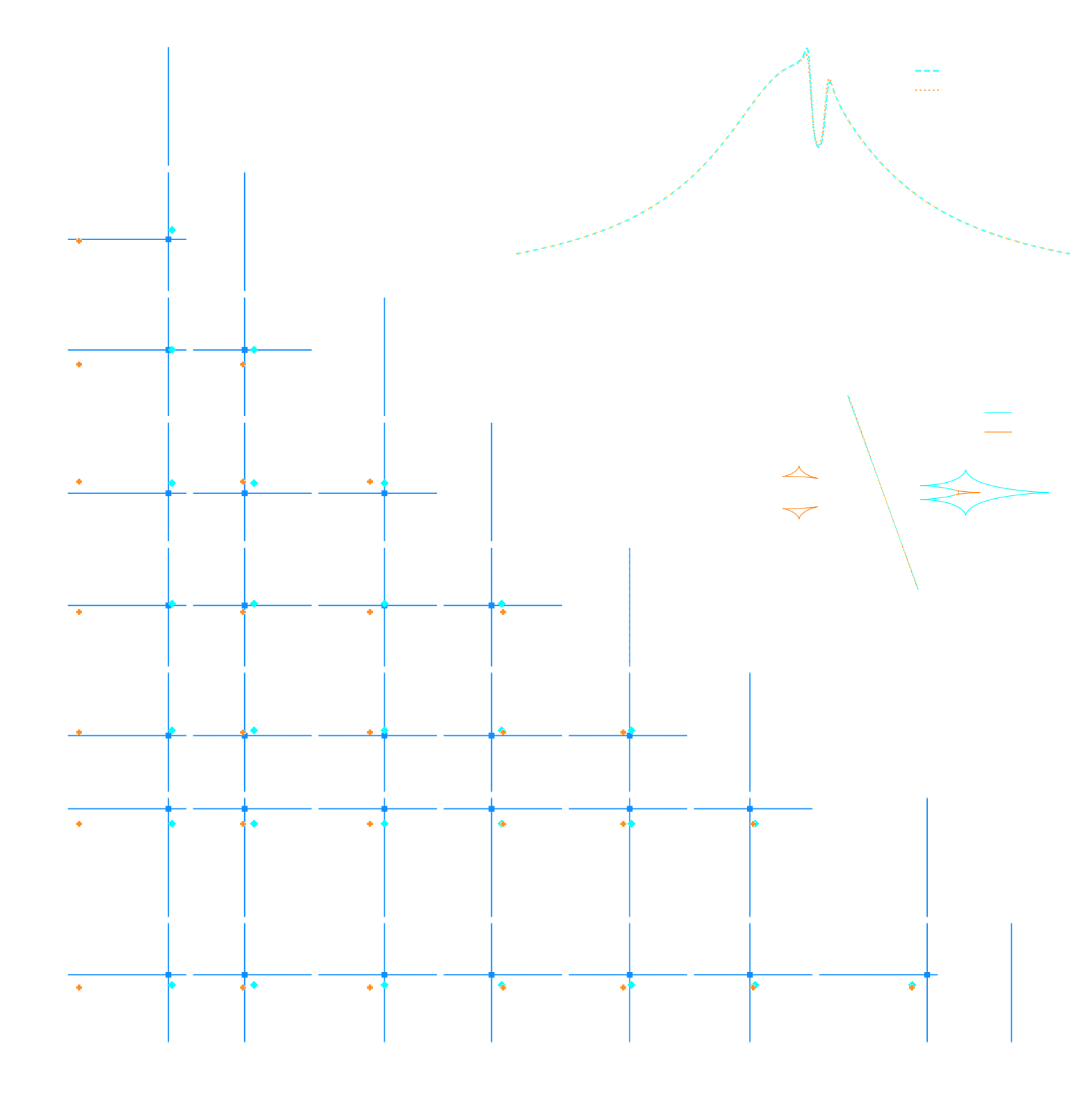
Example of application: Infering Microlensing Event Parameters
Example of application: Likelihood-Free parameter inference with DES SV
Suite of N-body + raytracing simulations: $\mathcal{D}$
Main takeaways
- This approach automatizes cosmological inference
- Turns the summary extraction and inference problems into an optimization problems
- If neural networks fail, inference will be sub-optimal but not necessarily biased.
- Some resources and links:
- Review on Simulation-Based Inference: Cranmer, Brehmer, Louppe (2020)
- Recent full $w$CDM Likelihood-Free Inference constraints on DES Y3: Fluri, Kacprzak, Lucchi, Schneider, Refregier, Hofmann (2022)
- Simulation Based Inference packages: sbi, pydelfy, Information Maximizing Neural Networks
Solving Ill-Posed Inverse Problems with Deep Learning
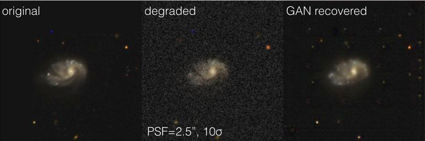
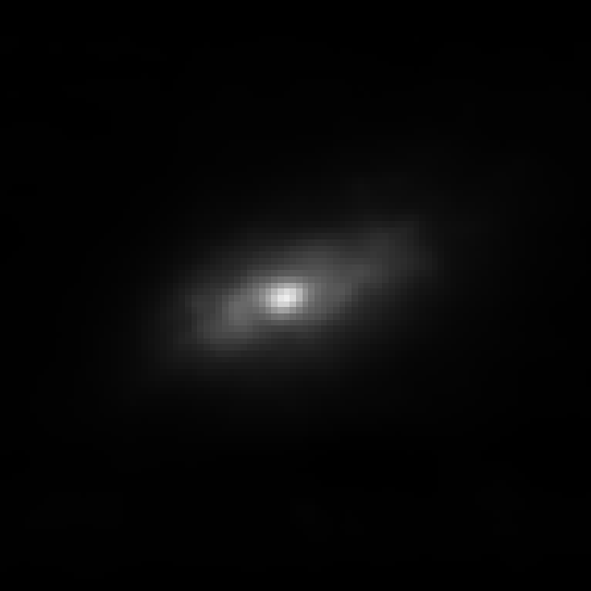
A motivating example: Image Deconvolution
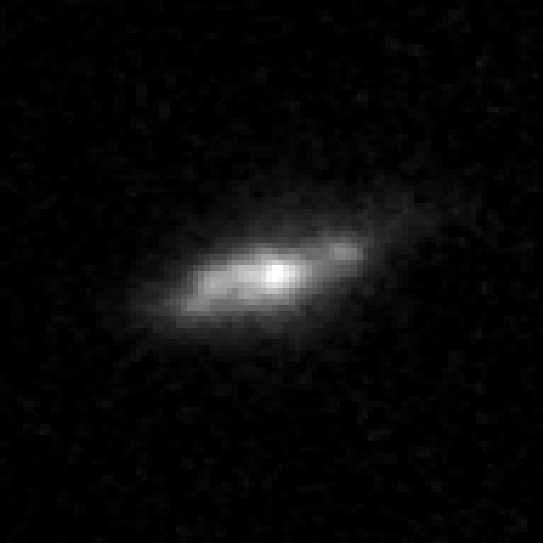
Hubble Space Telescope
some deep neural network
Simulated Ground-Based Telescope
- No explicit control of noise, PSF, depth.
- Unless covered by the training data, the result becomes unpredictable.
- No guarantees some physical properties are preserved
$\Longrightarrow$ In this case, the flux of the deconvolved object - Robust quantification of uncertainties is extremely difficult.
Example: GalaxyGAN (Schawinski et al. 2017)
Linear inverse problems
$\boxed{y = \mathbf{A}x + n}$$\mathbf{A}$ is known and encodes our physical understanding of the problem.
$\Longrightarrow$ When non-invertible or ill-conditioned, the inverse problem is ill-posed with no unique solution $x$
 Deconvolution
 Inpainting
 Denoising
A Bayesian view of the problem
$\boxed{y = \mathbf{A}x + n}$- $p(y | x)$ is the data likelihood, which contains the
physics
- $p(x)$ is our prior knowledge on the solution.
$$\hat{x} = \arg\max\limits_x \ \log p(y \ | \ x) + \log p(x)$$ For instance, if $n$ is Gaussian, $\hat{x} = \arg\max\limits_x \ - \frac{1}{2} \parallel y - \mathbf{A} x \parallel_{\mathbf{\Sigma}}^2 + \log p(x)$
How do you choose the prior ?
Classical examples of signal priors
$$ \log p(x) = \parallel \mathbf{W} x \parallel_1 $$
 $$ \log p(x) = x^t \mathbf{\Sigma^{-1}} x $$
But what about this?
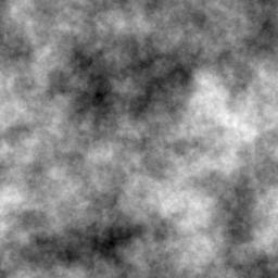
Maybe we can learn priors from the data!
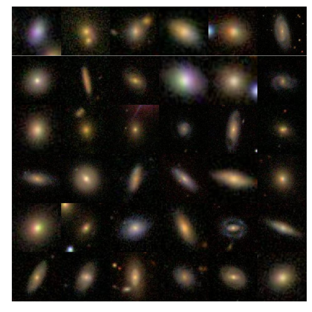
- The goal of generative modeling is to learn an implicit distribution $\mathbb{P}$ from which the training set $X = \{x_0, x_1, \ldots, x_n \}$ is drawn.
- Usually, this means building a parametric model $\mathbb{P}_\theta$ that tries to be close to $\mathbb{P}$.
True $\mathbb{P}$
Samples $x_i \sim \mathbb{P}$
Model $\mathbb{P}_\theta$
- Once trained, you can typically sample from $\mathbb{P}_\theta$ and/or evaluate the likelihood $p_\theta(x)$.
Why are these generative models useful?
Implicit distributions are everywhere!
Deep Generative Modeling
Why isn't it easy?
- The curse of dimensionality put all points far apart in high dimension


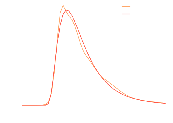
Distance between pairs of points drawn from a Gaussian distribution.
- Classical methods for estimating probability densities, i.e. Kernel Density Estimation (KDE) start to fail in high dimension because of all the gaps
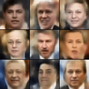
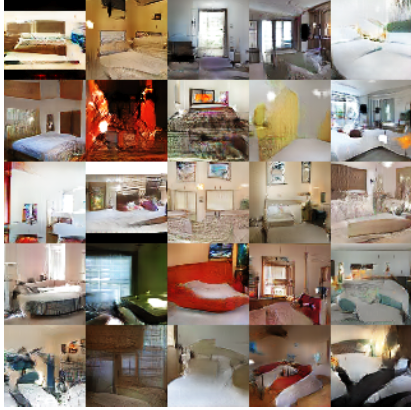
The evolution of generative models
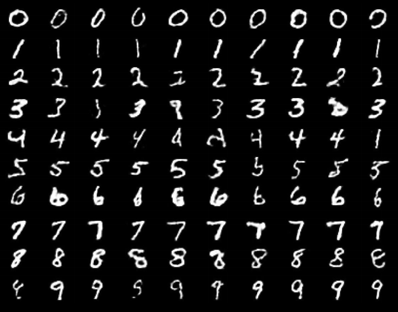
- Deep Belief Network
(Hinton et al. 2006) - Variational AutoEncoder
(Kingma & Welling 2014) - Generative Adversarial Network
(Goodfellow et al. 2014) - Wasserstein GAN
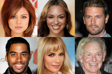
(Arjovsky et al. 2017) - Midjourney v5 Guided Diffusion (2023)
A visual Turing test
A brief survey of Generative Models Families

- Latent Variable Models:
Assume the following form for the model disribution: $$ x = f_\theta(z) \qquad \mbox{with} \qquad z \sim p(z)$$ This is the case of Generative Adversarial Networks, Variational Auto-Encoders, Normalizing Flows. - Auto-Regressive Models:
Assume an autoregressive decomposition of the signal into products of 1D conditional distributions: $$ p_\theta(x) = p_\theta(x_0) p_\theta(x_1 | x_0) \ldots p_\theta(x_n | x_{n-1}, \ldots x_{0}) $$ This is the case of PixelCNN, GPT-3 - Diffusion Models:
Target distribution generated by a reverse noise diffusion process controled by a Stochastic Differential Equation (SDE).
The Variational Auto-Encoder
- We assume a prior distribution $p(z)$ for the latent variable, and a likelihood $p_\theta(x |z)$ defined by a neural network.
Typically $p_\theta(x|z) = \mathcal{N}(x; f_\theta(x), \sigma^2)$ - Training the generative model amounts to finding $\theta_\star$ that
maximizes the marginal likelihood of the model:
$$p_\theta(x) = \int \mathcal{N}(x; f_\theta(z), \sigma^2) \ p(z) \ dz$$
$\Longrightarrow$ This is generally intractable
- In a VAE, efficient training of parameter $\theta$ is made possible by Amortized Variational Inference.
- We introduce a parametric distribution $q_\phi(z | x)$ which aims to model the posterior $p(z | x)$. We want to minimize $\mathbb{D}_{KL}\left( q_\phi(z | x) \parallel p(z | x) \right)$
- Working out the KL divergence between these two distributions leads to: $$\log p_\theta(x) \quad \geq \quad - \mathbb{D}_{KL}\left( q_\phi(z | x) \parallel p(z) \right) \quad + \quad \mathbb{E}_{z \sim q_{\phi}(. | x)} \left[ \log p_\theta(x | z) \right]$$ $\Longrightarrow$ This is the Evidence Lower-Bound, which is differentiable with respect to $\theta$ and $\phi$.
The famous Variational Auto-Encoder
$$\log p_\theta(x) \geq - \underbrace{\mathbb{D}_{KL}\left( q_\phi(z | x) \parallel p(z) \right)}_{\mbox{code regularization}} + \underbrace{\mathbb{E}_{z \sim q_{\phi}(. | x)} \left[ \log p_\theta(x | z) \right]}_{\mbox{reconstruction error}} $$
Normalizing Flows
Still a latent variable model, except the mapping $f_\theta$ is made to be bijective.
- Assumes a bijective mapping between data space $x$ and latent space $z$ with prior $p(z)$: $$ z = f_{\theta} ( x ) \qquad \mbox{and} \qquad x = f^{-1}_{\theta}(z)$$
- Admits an explicit marginal likelihood: $$ \log p_\theta(x) = \log p(z) + \log \left| \frac{\partial f_\theta}{\partial x} \right|(x) $$
One example of NF: RealNVP
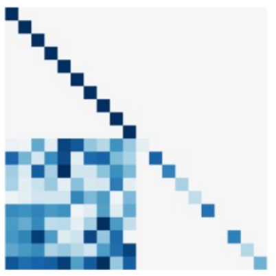
Jacobian of an affine coupling layer
We will call this layer an affine coupling.
$\Longrightarrow$ This structure has the advantage that the Jacobian of this layer will be lower triangular which makes computing its determinant easy.
Not all generative models are created equal
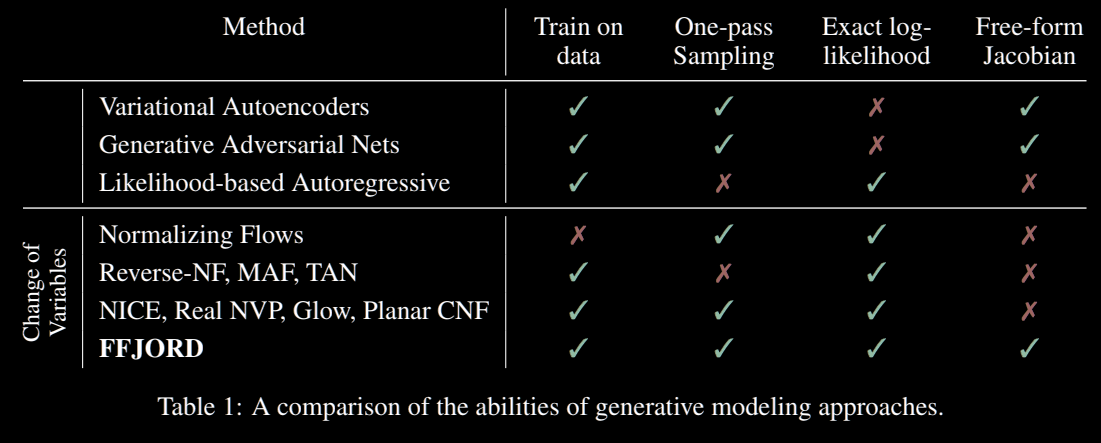
- Of particular interest are models with an explicit $\log p(x)$ (not the case of VAEs, GANs, Denoising Diffusion Models).
Your Turn!
We will be using this notebook to implement a Normalizing Flow in JAX+Flax+TensorFlow Probability
Application to
Solving Inverse Problems
Getting started with Deep Priors: deep denoising example
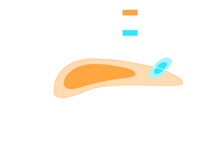
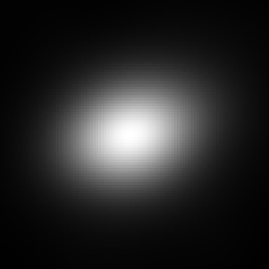
$$ \boxed{{\color{Orchid} y} = {\color{SkyBlue} x} + n} $$
- Let us assume we have access to examples of $ {\color{SkyBlue} x}$ without noise.
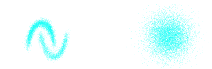
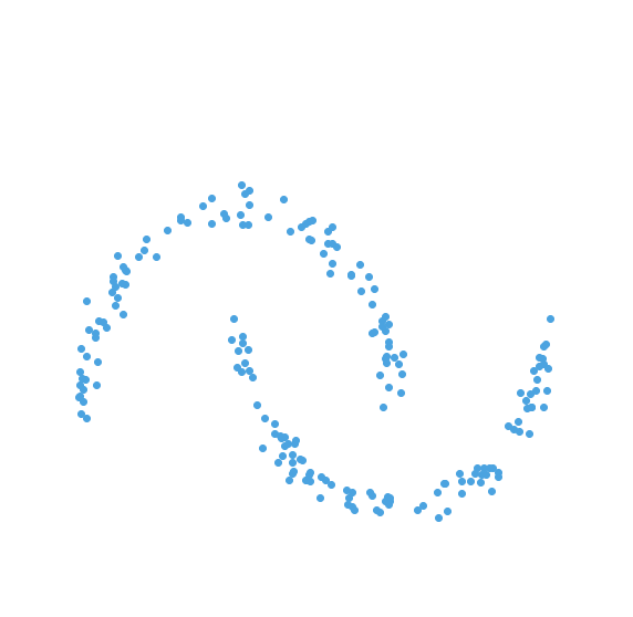
- We learn the distribution of noiseless data $\log p_\theta(x)$ from samples using a deep generative model.
- The solution should lie on the realistic data
manifold, symbolized by the two-moons distribution.
We want to solve for the Maximum A Posterior solution:
$$\arg \max - \frac{1}{2} \parallel {\color{Orchid} y} - {\color{SkyBlue} x} \parallel_2^2 + \log p_\theta({\color{SkyBlue} x})$$ This can be done by gradient descent as long as one has access to the score function $\frac{\color{orange} d \color{orange}\log \color{orange}p\color{orange}(\color{orange}x\color{orange})}{\color{orange} d \color{orange}x}$.
A Physicist's approach to the deconvolution problem: let's build a model

$g_\theta$
PSF
Pixelation
Noise
latent $z$ is a denoised galaxy image
latent $z$ is a super-resolved and denoised galaxy image
latent $z$ is a deconvolved, super-resolved, and denoised galaxy image
latent $z$ is a Gaussian sample
$\theta$ are parameters of the model
Bayesian Inference a.k.a. Uncertainty Quantification
- $p( z | x )$ is the posterior
- $p( x | z )$ is the data likelihood, contains the physics
- $p( z )$ is the prior
$x_n$
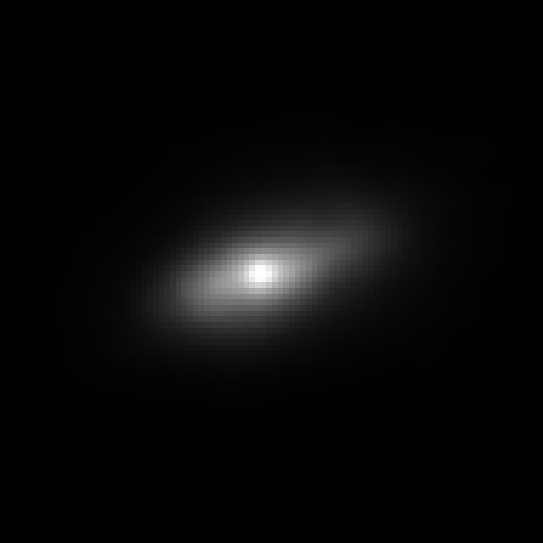
$x_0$
$g_\theta(z)$
$\mathbf{P} (\Pi \ast g_\theta(z))$
$x_n - \mathbf{P} (\Pi \ast g_\theta(z))$
Now you try it!
We will be using this notebook: https://tinyurl.com/inverse-problemYour goal: Solve an image deconvolution problem using a deep generative model as a prior.
Raise your hand when you reach the Maximum Likelihood Solution i.e. end of Step III.
How to solve the posterior inference problem by Variational Inference?
- The core idea of Variational Inference is to assume a model distribution $q_\phi$ and we fit it to the unknown posterior.
- How do we fit a distribution to another distribution? We minize the KL divergence $$ \mathbb{D}_{KL}\left( q_\phi(z) \parallel p(z | x) \right) = \mathbb{E}_{z \sim q_{\phi}} \left[ \log \frac{q_\phi(z)}{p(z | x)} \right] $$$$ = \mathbb{E}_{z \sim q_{\phi}} \left[ \log q(z) \right] - \mathbb{E}_{z \sim q_{\phi}} \left[ \log p(z | x) \right] $$$$ = \mathbb{E}_{z \sim q_{\phi}} \left[ \log q(z) \right] - \mathbb{E}_{z \sim q_{\phi}} \left[ \log p(x | z) + \log p(z) - \log p(x)\right] $$$$ = \underbrace{\mathbb{D}_{KL}\left( q_\phi(z) \parallel p(z) \right) - \mathbb{E}_{z \sim q_{\phi}} \left[ \log p(x | z) \right]}_{\mbox{Evidence Lower Bound}} + \log p(x) $$
- Finally, we need a flexible enough model distribution, why not a Normalizing Flow :-) ?
Example of Application at Scale
Let's set the stage: Gravitational lensing
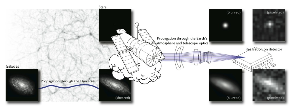
- We are trying the measure the ellipticity $e$ of galaxies as an estimator for the gravitational shear $\gamma$
Gravitational Lensing as an Inverse Problem
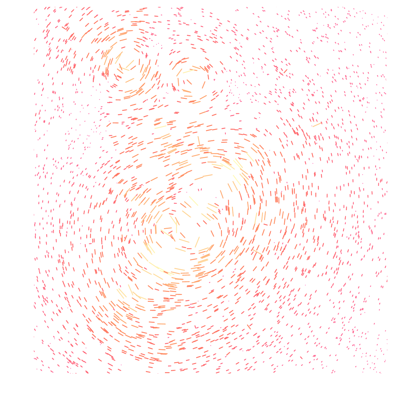
Writing down the convergence map log posterior
$$ \log p( \kappa | e) = \underbrace{\log p(e | \kappa)}_{\simeq -\frac{1}{2} \parallel e - P \kappa \parallel_\Sigma^2} + \log p(\kappa) +cst $$- The likelihood term is known analytically, given to us by the physics of gravitational lensing.
- There is no close form expression for the prior on dark matter maps $\kappa$.
However:- We do have access to samples of full implicit prior through simulations: $X = \{x_0, x_1, \ldots, x_n \}$ with $x_i \sim \mathbb{P}$
![]()
- We do have access to samples of full implicit prior through simulations: $X = \{x_0, x_1, \ldots, x_n \}$ with $x_i \sim \mathbb{P}$
How do you do this in practice in very high dimensional problems?
First realization: The score is all you need!
- Whether you are looking for the MAP or sampling with HMC or MALA, you
only need access to the score of the posterior:
$$\frac{\color{orange} d \color{orange}\log \color{orange}p\color{orange}(\color{orange}x \color{orange}|\color{orange} y\color{orange})}{\color{orange}
d
\color{orange}x}$$
- Gradient descent: $x_{t+1} = x_t + \tau \nabla_x \log p(x_t | y) $
- Langevin algorithm: $x_{t+1} = x_t + \tau \nabla_x \log p(x_t | y) + \sqrt{2\tau} n_t$
- The score of the full posterior is simply: $$\nabla_x \log p(x |y) = \underbrace{\nabla_x \log p(y |x)}_{\mbox{known explicitly}} \quad + \quad \underbrace{\nabla_x \log p(x)}_{\mbox{known implicitly}}$$ $\Longrightarrow$ "all" we have to do is model/learn the score of the prior.
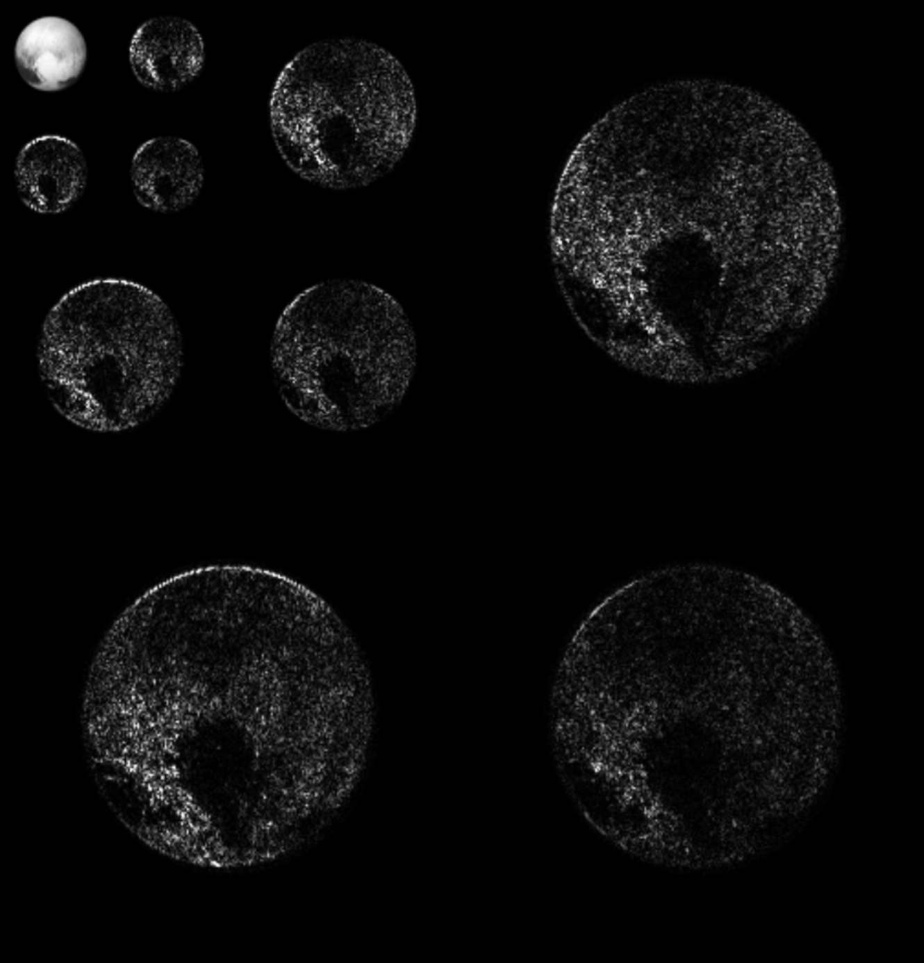
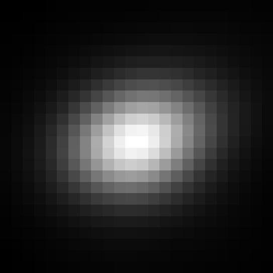
Neural Score Estimation by Denoising Score Matching (Vincent 2011)
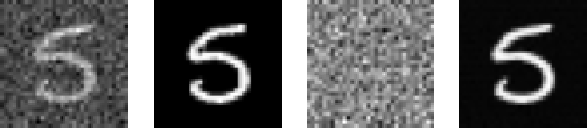
- Denoising Score Matching: An optimal Gaussian denoiser learns the score of a given distribution.
- If $x \sim \mathbb{P}$ is corrupted by additional Gaussian noise $u \in \mathcal{N}(0, \sigma^2)$ to yield $$x^\prime = x + u$$
- Let's consider a denoiser $r_\theta$ trained under an $\ell_2$ loss: $$\mathcal{L}=\parallel x - r_\theta(x^\prime, \sigma) \parallel_2^2$$
- The optimal denoiser $r_{\theta^\star}$ verifies: $$\boxed{\boldsymbol{r}_{\theta^\star}(\boldsymbol{x}', \sigma) = \boldsymbol{x}' + \sigma^2 \nabla_{\boldsymbol{x}} \log p_{\sigma^2}(\boldsymbol{x}')}$$
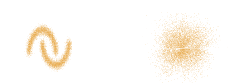
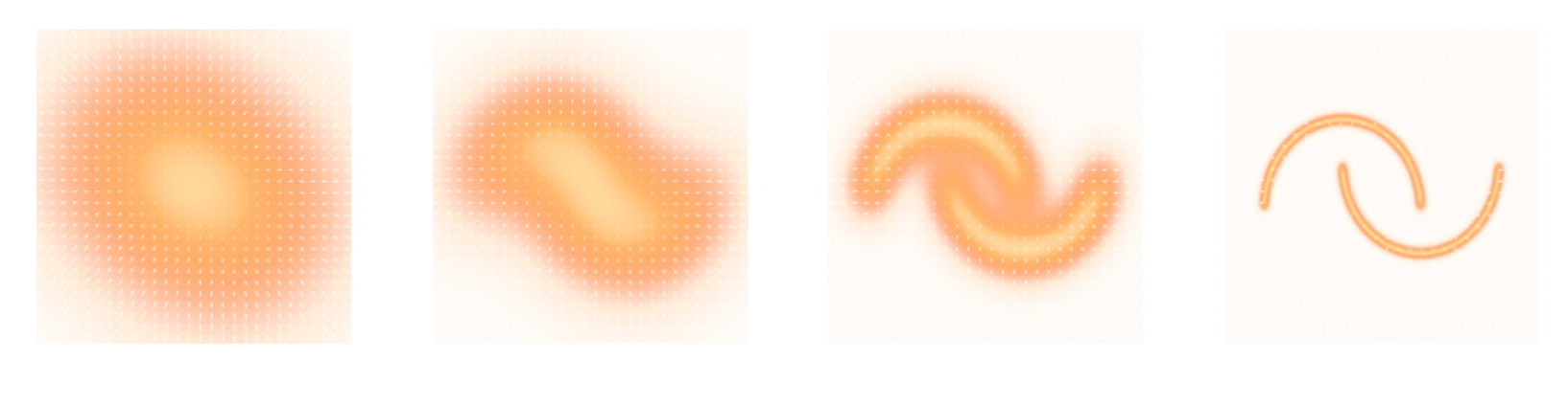
Second Realization: Annealing is everything!
- Even with knowledge of the score, sampling in high number of dimensions is difficult!
- Convolving a target distribution $p$ with a noise kernel, makes $p_\sigma(x) = \int \mathcal{N}(x; x^\prime, \sigma^2) (x^\prime) d x^{\prime}$ it much better behaved
$$\sigma_1 > \sigma_2 > \sigma_3 > \sigma_4 $$
![]()
- Hints to running many MCMC chains in parallel, progressively annealing the $\sigma$ to 0, keep last point in the chain as independent sample.
Score-Based Generative Modeling Song et al. (2021)
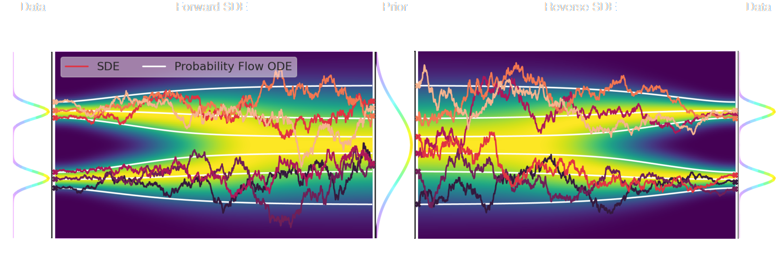
- The SDE defines a marginal distribution $p_t(x)$ as the convolution of the target distribution $p(x)$ with a noise kernel $p_{t|s}(\cdot | x_s)$: $$p_t(x) = \int p(x_s) p_{t|s}(x | x_s) d x_s$$
- For a given forward SDE that evolves $p(x)$ to $p_T(x)$, there exists a reverse SDE that evolves $p_T(x)$ back into $p(x)$. It involves having access to the marginal score $\nabla_x \log_t p(x)$.
Example of one chain during annealing
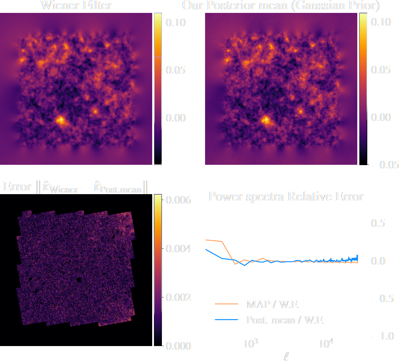
Validating Posterior Sampling under a Gaussian prior
Some details: We don't actually know the marginal posterior score!
- We know the following quantities:
- Annealed likelihood (analytically): $p_\sigma(y | x) = \mathcal{N}(y; \mathbf{A} x, \mathbf{\Sigma} + \sigma^2 \mathbf{I})$
- Annealed prior score (by score matching): $\nabla_x \log p_\sigma(x)$
- But, unfortunately: $\boxed{p_\sigma(x|y) \neq p_\sigma(y|x) \ p_\sigma(x)}$ $\Longrightarrow$ We don't know the marginal posterior score!
- We cannot use the reverse SDE/ODE of diffusion models to sample from the posterior. $$\mathrm{d} x = [f(x, t) - g^2(t) \underbrace{\nabla_x \log p_t(x|y)}_{\mbox{unknown}} ] \mathrm{d}t + g(t) \mathrm{d} w$$
- Even if not equivalent to the marginal posterior score, $\nabla_x \log p_{\sigma^2}(y | x) + \nabla_x \log p_{\sigma^2}(x)$ still
has good properties:
- Tends to an isotropic Gaussian distribution for large $\sigma$
- Corresponds to the target posterior for $\sigma=0$
- If we simulate this SDE sufficiently slowly (i.e. timescale of change of $\sigma$ is much larger than the timescale of the SDE) we can expect to sample from the target posterior.
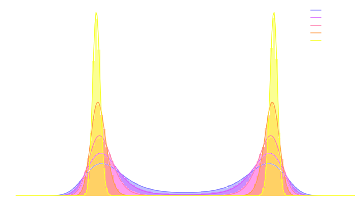
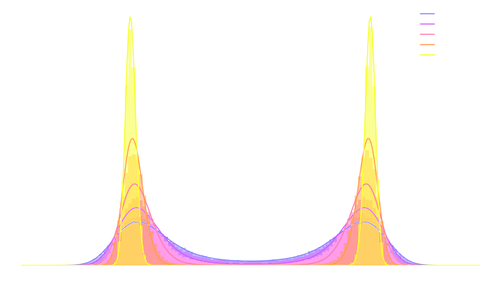
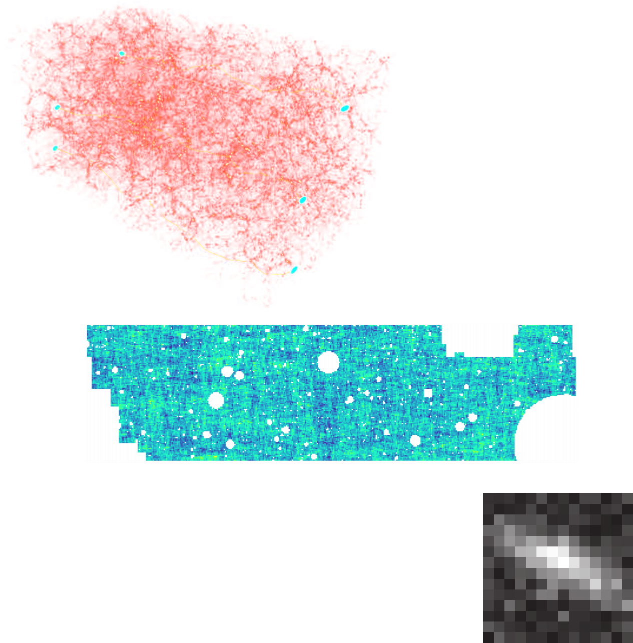
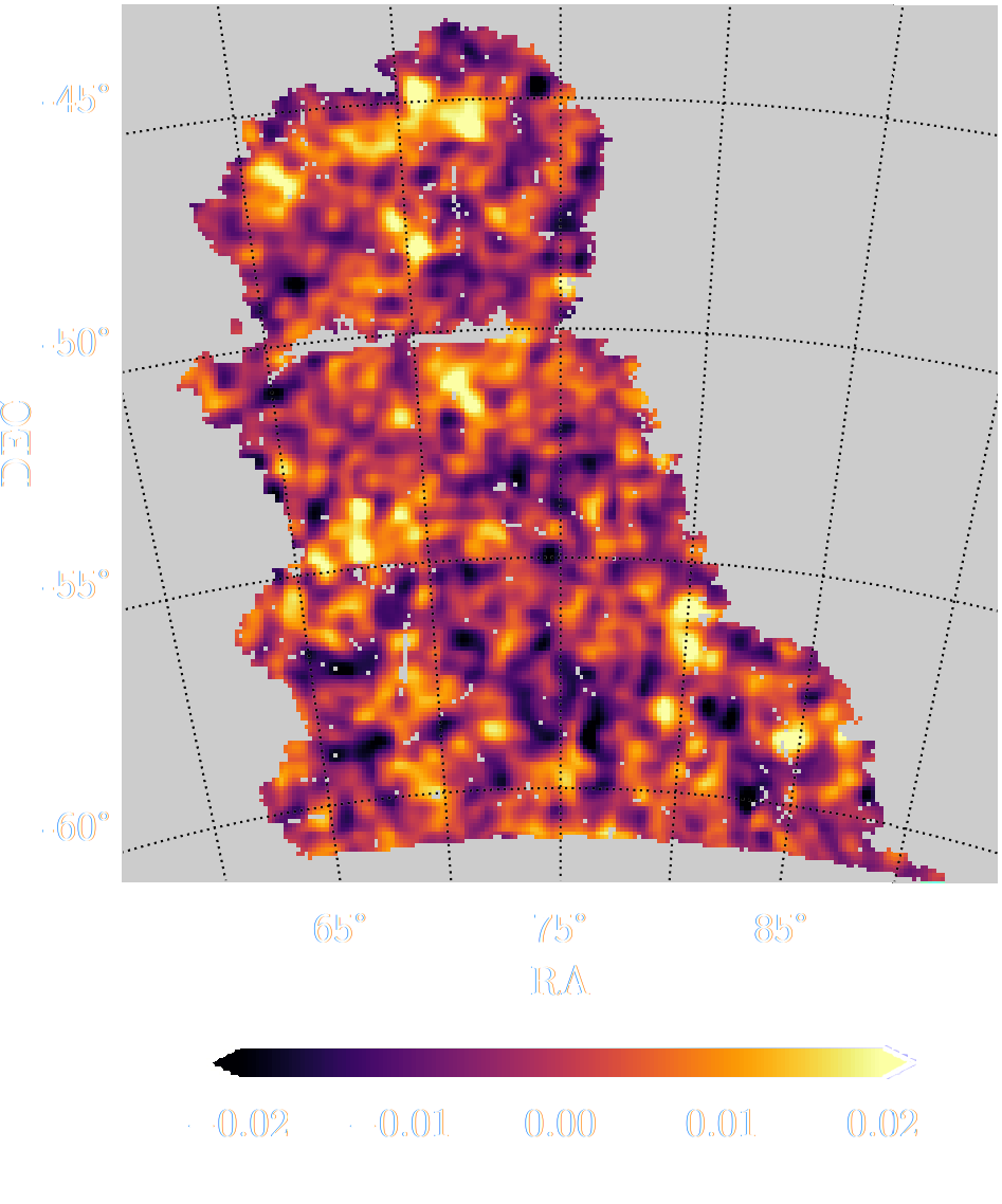
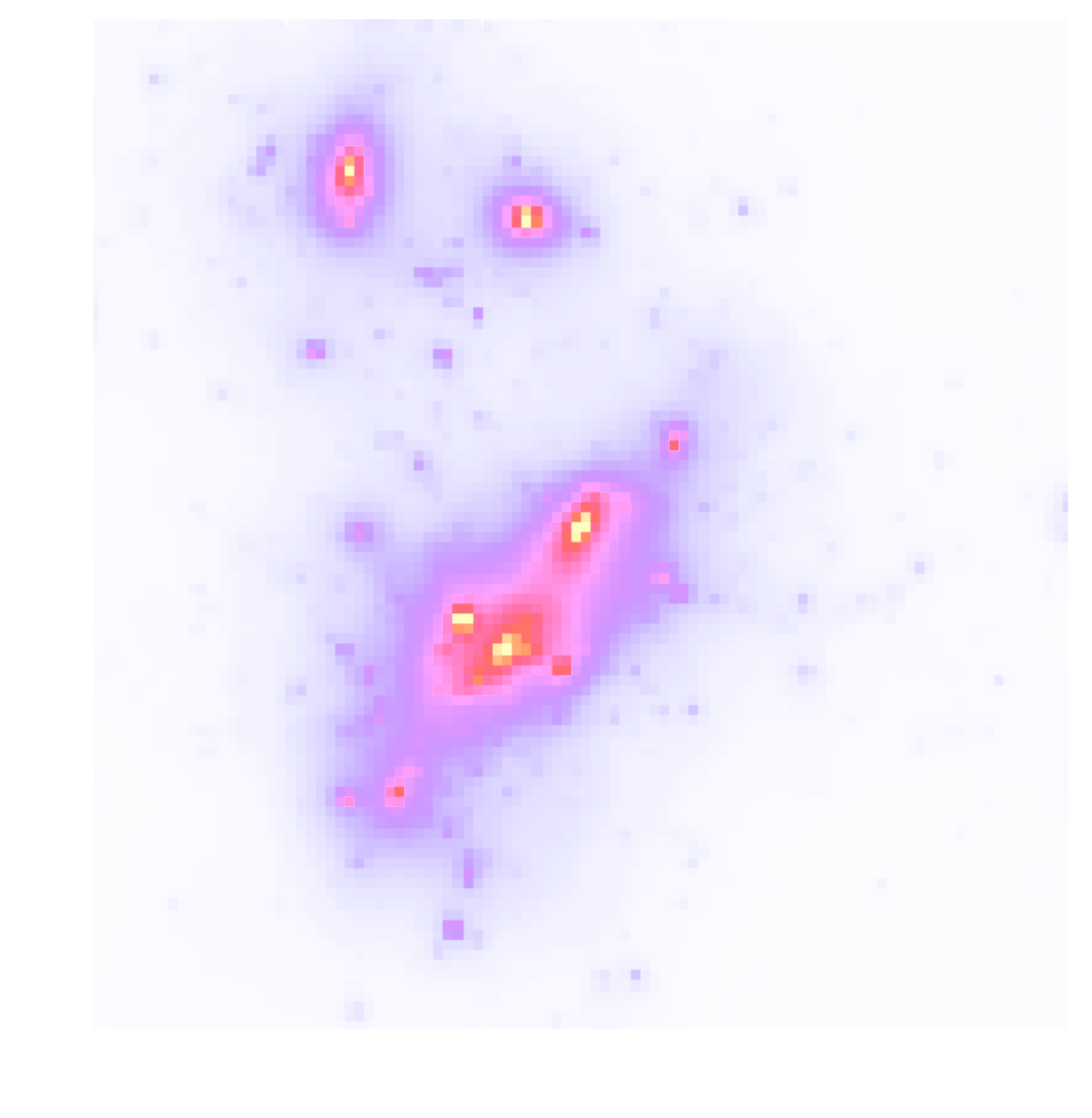
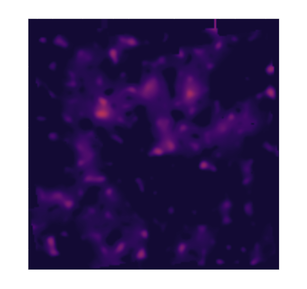
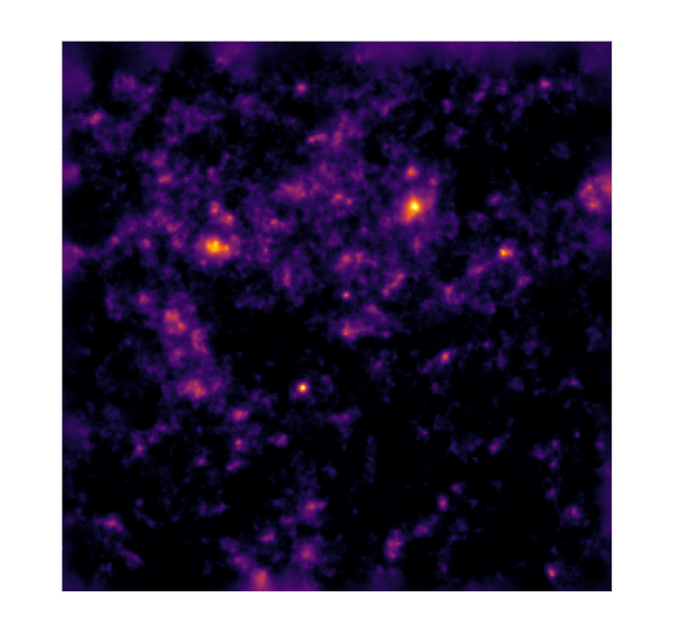
Illustration on $\kappa$-TNG simulations
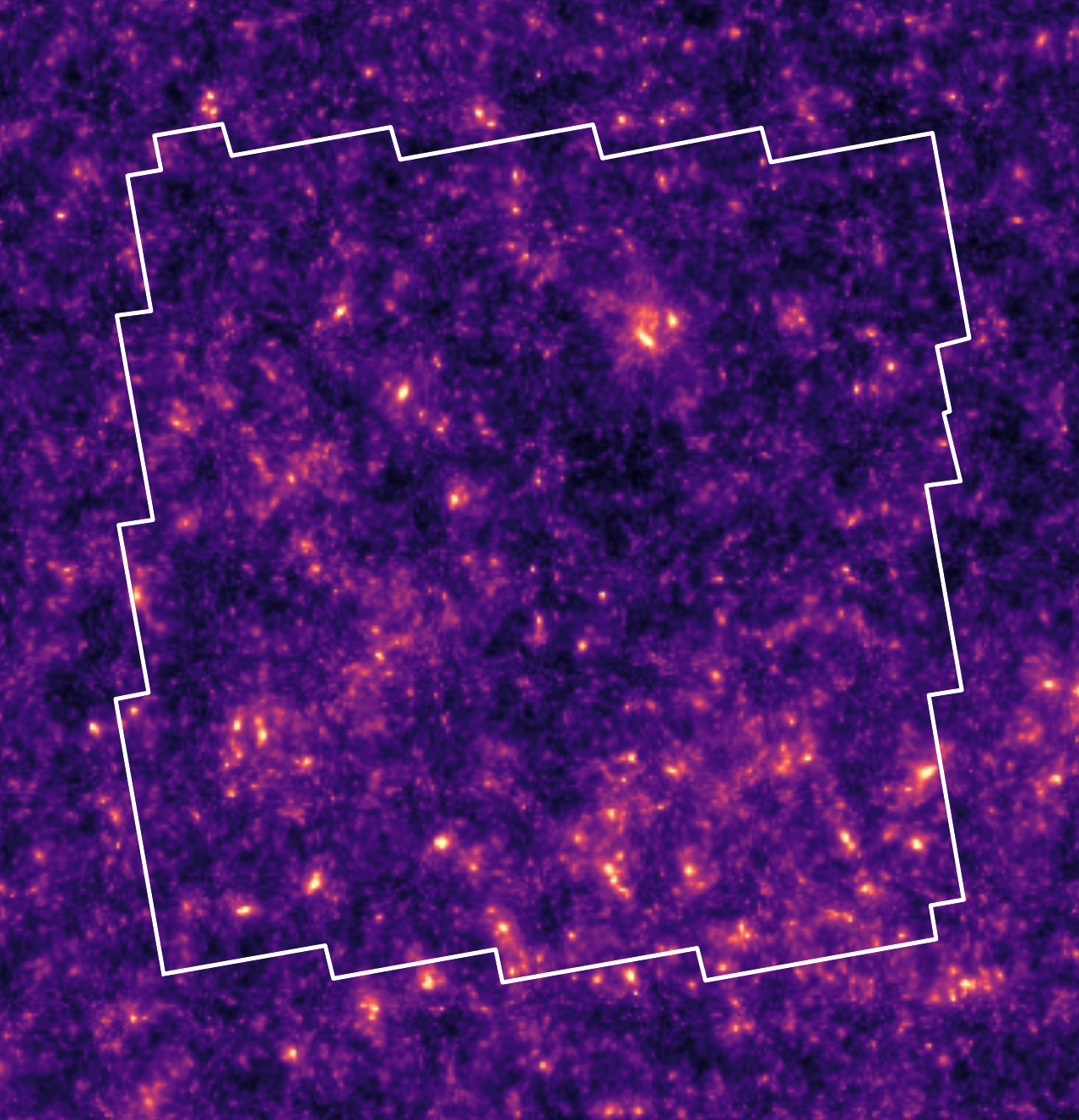
True convergence map
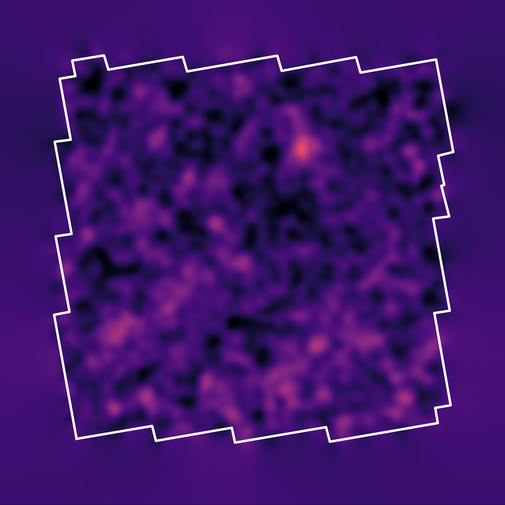
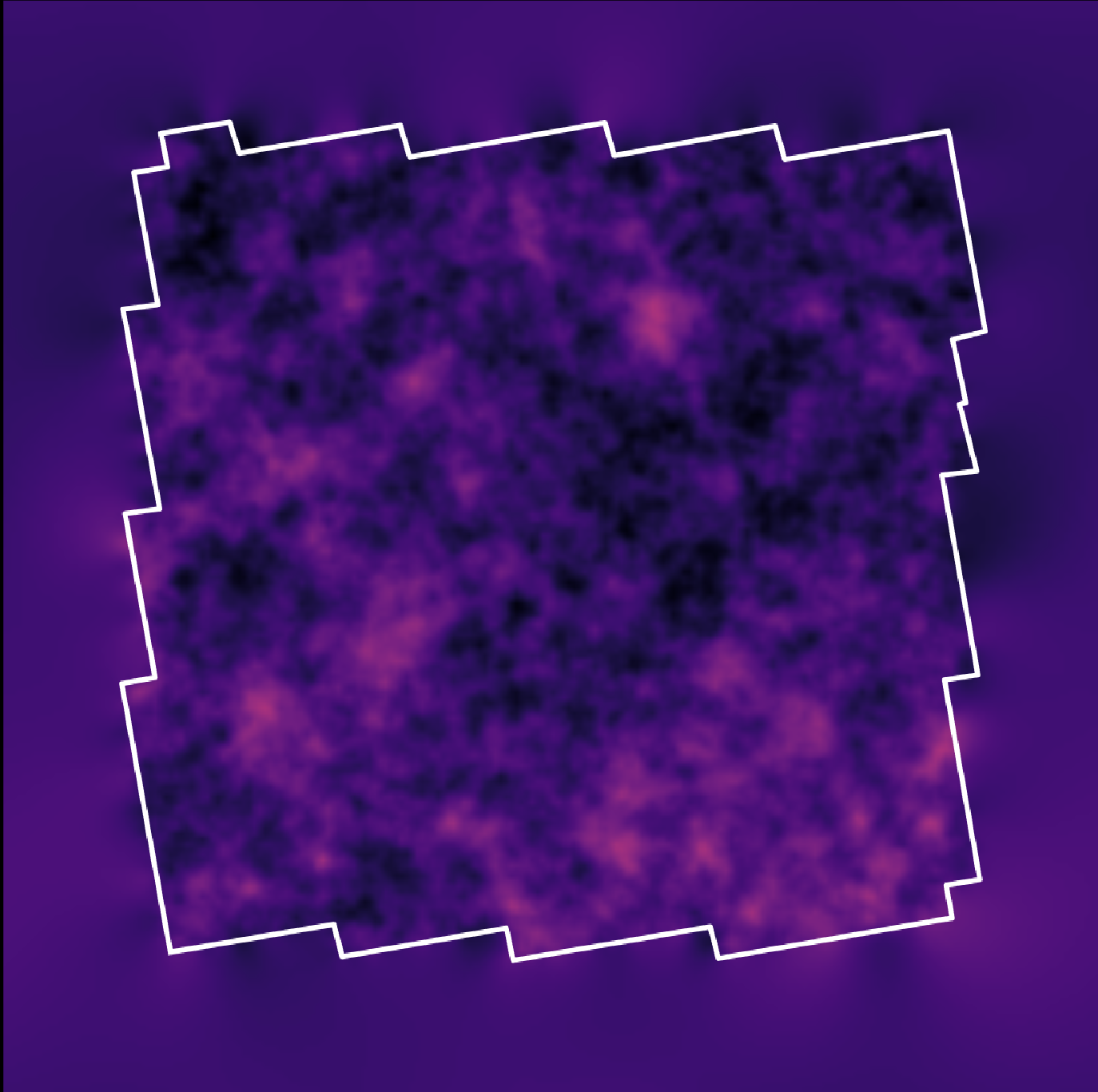
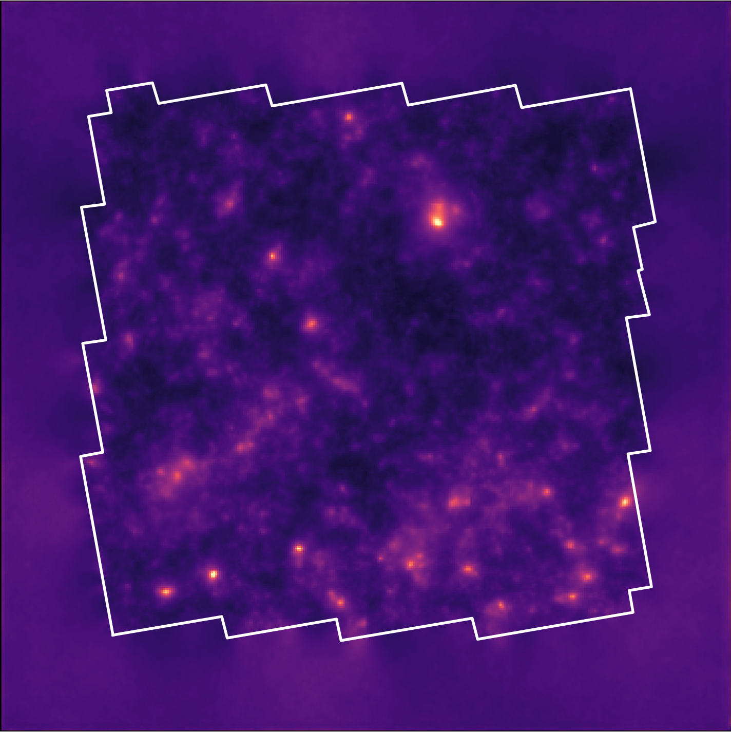
Posterior samples
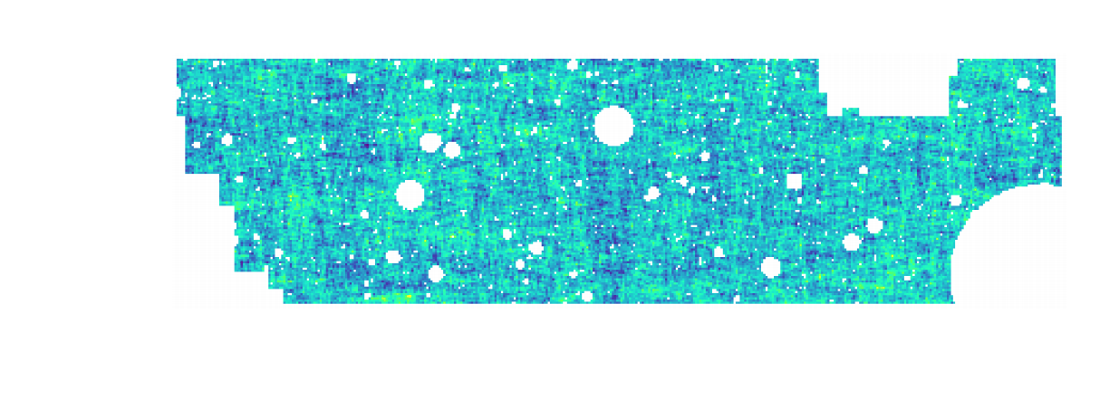
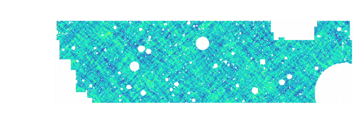
Reconstruction of the HST/ACS COSMOS field
- COSMOS shear data from Schrabback et al. 2010
- Prior learned from $\kappa$-TNG simulation from Osato et al. 2021.
Other examples of Deep Priors
- Hybrid Physical-Deep Learning Model for Astronomical Inverse Problems
F. Lanusse, P. Melchior, F. Moolekamp

$\mathcal{L} = \frac{1}{2} \parallel \mathbf{\Sigma}^{-1/2} (\ Y - P \ast A S \ ) \parallel_2^2 - \sum_{i=1}^K \log p_{\theta}(S_i)$

- Denoising Score-Matching for Uncertainty Quantification in Inverse Problems
Z. Ramzi, B. Remy, F. Lanusse, P. Ciuciu, J.L. Starck